Are you looking to apply the SVM classifier using Python on a classification dataset? Here we go!
The support Vector Machine (SVM Classifier) algorithm is a Machine Learning algorithm that analyzes data for classification and regression, but its real strength is in solving classification problems. It can be used for binary and multi-class classification. In this article, we will discuss the Support Vector Machine and will learn how to implement it on a classification problem. We will also, evaluate and visualize the results. For the evaluation purposes of the SVM classifier, we will be using a confusion matrix, recall, precision, and accuracy. Moreover, we will use various visualization tools in order to visualize the SVM-trained model and predictions.
What is an SVM Classifier in Sklearn?
Support Vector Machine (SVM Classifier), also known as Support Vector Classification, is a supervised and linear Machine Learning technique typically used to solve classification problems. SVR stands for Support Vector Regression and is a subset of SVM that uses the same ideas to tackle regression problems. SVM also supports the kernel method called the kernel SVM, which allows us to tackle non-linearity.
Now lets us explain some of the important terms that are frequently used in the SVM Classifier algorithm.
- Support Vectors are data points closest to the hyperplane called support vectors. These points will define the separating line better by calculating margins and are more relevant to the construction of the classifier.
- A hyperplane is a decision plane that separates a set of objects having different class memberships.
- Margin is the distance between the two lines on the class points closest to each other. It is calculated as the perpendicular distance from the line to support vectors or nearest points. The bold margin between the classes is good, whereas a thin margin is not good.
Depending on the type of data, there are two types of Support Vector Machines:
- Linear SVM or Simple SVM is used for data that is linearly separable. A dataset is termed linearly separable data if it can be classified into two classes using a single straight line, and the classifier is known as the linear machine learning SVM classifier. It’s most commonly used for tasks involving linear regression and classification.
- Nonlinear SVM or Kernel SVM also known as Kernel SVM, is a type of machine learning SVM that is used to classify nonlinearly separated data or data that cannot be classified using a straight line. It has more flexibility for nonlinear data because more features can be added to fit a hyperplane instead of a two-dimensional space.
In the upcoming section, we will use both types of SVM classifiers to classify the given dataset.
How Does the SVM Algorithm Works?
To understand the working of the SVM algorithm, let us take a simple classification example. Let us say we want to know how the machine learning SVM Classifier will classify animals into cat or dog categories. The classification will be based on the characteristics of the animals we provide to the machine. For example, it can be the animals’ size, shape, color, or weight. The more features we consider, the easier it is to identify and distinguish both.
The objective of machine learning SVM is to draw a line that best separates the two classes of data points. So, the SVM produces a line that cleanly divides the two classes. There are many other ways to construct a line that separates the two classes, but in machine learning SVM, the margins and support vectors are used.
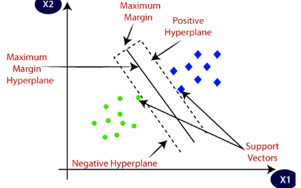
As shown in the image above, the margin is the area separating the two dotted lines. The larger this margin is, the better the classifier will be. The data points that each dotted line passes through are the support vectors. These points are known as support vectors since they help define the margins and the classifier. These support vectors are the data points closest to the border of either of the classes and have a chance of belonging to one of them.
Support Vector Machine Using Python
Now we will use the machine learning SVM Classifier to classify a binary dataset. The dataset is about costumer and whether they purchased the term or not based on their age and salary. You can access the dataset and the Jupyter Notebook from my GitHub account. Here we will explain each part of the code in detail.
But before going to the implementation part, make sure that you have installed the following required Python modules.
- sklearn
- pandas
- NumPy
- matplotlib
- plotly
- seaborn
You can use the pip command to install the required modules.
Exploring Dataset For SVM Classifier
Let us first import the dataset using pandas and print out a few rows.
# importing pandas
import pandas as pd

# improting dataset
data = pd.read_csv('dataset.csv')

# heading of dataset
data.head()
As you can see, we have two input columns and one output column. The input columns are about the age and salary of a person and the target class is whether that person purchased the product or not.
Let us now see the total number of people who purchased and who didn’t by plotting a bar plot.
import seaborn as sns
sns.countplot(data, x='Purchased')
Output:
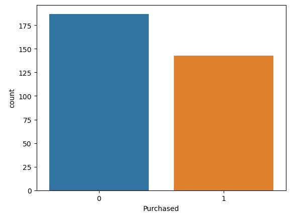
As you can see we have nearly 180 people who didn’t purchase the item and nearly 145 people who purchased it.
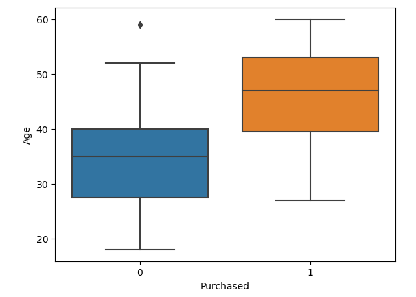
Now, let us also use the box plot to find the distribution of the input variables. A box plot is a simple way of representing statistical data on a plot in which a rectangle is drawn to represent the second and third quartiles, usually with a vertical line inside to indicate the median value. The lower and upper quartiles are shown as horizontal lines on either side of the rectangle.
For example, below are two box plots showing the distribution of age attributes of who purchased the item and who didn’t.
# ploting box graph ( age and success)
sns.boxplot(data, y=data["Age"], x=data['Purchased'])
Output:
Splitting Dataset
Before splitting the dataset into testing and training parts, we will divide the dataset into input and output values.
# dividing the dataset for Support Vector Machine using Python
X = data.drop('Purchased', axis=1)
y = data['Purchased']
Now, we will split the dataset into testing and training parts. We will also assign a value of 0 to the random state.
# importing the train_test_split method from sklearn
from sklearn.model_selection import train_test_split

# splitting the data
X_train, X_test, y_train, y_test = train_test_split(X, y, test_size=0.30, random_state=0)
Once the splitting is complete, we can then go to the training of the model. If your dataset contains non-numeric values, then you can use encoding methods to convert the non-numeric values to numeric values.
Training the SVM Classifier With Linear Kernel
Linear Kernel is a regular dot product for two observations. The sum of the multiplication of each pair of input values is the product of two vectors. First, let us train our model using a linear kernel.
# importing Support Vector Machine using Python
from sklearn.svm import SVC

# kernelSupport Vector Machine using Python
classifier = SVC(kernel='linear')

# trainin Support Vector Machine using Python
classifier.fit(X_train, y_train)
Once the training is complete, we can then use the model to make predictions using the testing dataset.
# testing Support Vector Machine using Python
y_pred = classifier.predict(X_test)
Before going to the evaluation of the model, let us first visualize the machine learning SVM model which was trained using a linear kernel.
Visualizing SVM Classifier Trained Model
We will use matplotlib module to visualize the trained model.
# importing the modules
import numpy as np
import matplotlib.pyplot as plt
from matplotlib.colors import ListedColormap

# plotting the fgiure
plt.figure(figsize = (7,7))

# assigning the input values
X_set, y_set = X_train, y_train

# ploting the linear graph
X1, X2 = np.meshgrid(np.arange(start = X_set[:, 0].min() - 1, stop = X_set[:, 0].max() + 1, step = 0.01), np.arange(start = X_set[:, 1].min() - 1, stop = X_set[:, 1].max() + 1, step = 0.01))
plt.contourf(X1, X2, classifier.predict(np.array([X1.ravel(), X2.ravel()]).T).reshape(X1.shape), alpha = 0.75, cmap = ListedColormap(('black', 'white')))
plt.xlim(X1.min(), X1.max())
plt.ylim(X2.min(), X2.max())

# ploting scattered graph for the values
for i, j in enumerate(np.unique(y_set)):
    plt.scatter(X_set[y_set == j, 0], X_set[y_set == j, 1], c = ListedColormap(('red', 'blue'))(i), label = j)

# labeling the graph
plt.title('Purchased Vs Non-Purchased')
plt.xlabel('Salay')
plt.ylabel('Age')
plt.legend()
plt.show()
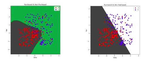
As you can see, the linear kernel has divided the dataset linearly.
Evaluating the SVM Classifier Model
Now, we will use the confusion matrix to find the ratio of the correctly classified and incorrectly classified items.
You may like: KNN algorithm in Sklearn
# importing the required modules
import matplotlib.pyplot as plt
from sklearn.metrics import confusion_matrix, ConfusionMatrixDisplay

# Plot the confusion matrix in graph
cm = confusion_matrix(y_test,y_pred, labels=classifier.classes_)

# ploting with labels
disp = ConfusionMatrixDisplay(confusion_matrix=cm, display_labels=classifier.classes_)
disp.plot()

# showing the matrix
plt.show()
Output:
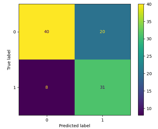
As you can see, the linear kernel was not able to predict most of the output values correctly. Let us also find the accuracy of the model.
# importing accuracy score
from sklearn.metrics import accuracy_score

# printing the accuracy score
accuracy_score(y_test,y_pred)
Output:
0.71717171717
As you can see, we get an accuracy score of 71% which means our model was able to classify 71% of the testing data correctly.
SVM Classifier Using Radial Basis Function Kernel
As we have seen we didn’t get a good accuracy score when using the linear kernel function. This time we will use the radial basis kernel function.
# kernel to be set radial bf
classifier1 = SVC(kernel='rbf')

# traininf Support Vector Machine using Python
classifier1.fit(X_train, y_train)

# testing Support Vector Machine using Python
y_pred = classifier1.predict(X_test)
As you can see, we have trained the model using the radial basis function. Let us now visualize the trained model as well.
Visualizing SVM-trained Model
Let us now visualize the trained model.
# plotting the fgiure
plt.figure(figsize = (7,7))

# assigning the input values
X_set, y_set = X_train, y_train

# ploting the linear graph / svm models
X1, X2 = np.meshgrid(np.arange(start = X_set[:, 0].min() - 1, stop = X_set[:, 0].max() + 1, step = 0.01), np.arange(start = X_set[:, 1].min() - 1, stop = X_set[:, 1].max() + 1, step = 0.01))
plt.contourf(X1, X2, classifier1.predict(np.array([X1.ravel(), X2.ravel()]).T).reshape(X1.shape), alpha = 0.75, cmap = ListedColormap(('black', 'green')))
plt.xlim(X1.min(), X1.max())
plt.ylim(X2.min(), X2.max())

# ploting scattered graph for the values
for i, j in enumerate(np.unique(y_set)):
    plt.scatter(X_set[y_set == j, 0], X_set[y_set == j, 1], c = ListedColormap(('red', 'blue'))(i), label = j)

# labeling the graph
plt.title('Purchased Vs Non-Purchased')
plt.xlabel('Salay')
plt.ylabel('Age')
plt.legend()
plt.show()
As you can see, this time the trained model is much more accurate.
Evaluating the SVM Model
Now, let us evaluate the performance of the model that was trained using the radial basis kernel function. We will again plot the confusion matrix of the model.
# Plot the confusion matrix in graph
cm = confusion_matrix(y_test,y_pred, labels=classifier.classes_)

# ploting with labels
disp = ConfusionMatrixDisplay(confusion_matrix=cm, display_labels=classifier.classes_)
disp.plot()

# showing the matrix
plt.show()
Output:
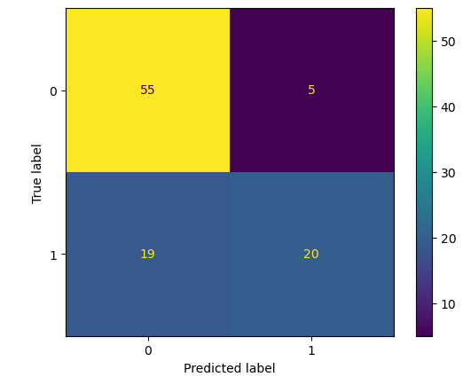
Let us also find the accuracy score of the model.
# printing the accuracy score
accuracy_score(y_test,y_pred)
Output:
0.7575757575
As you can see, we this a slightly better accuracy score this time.
Summary
Machine learning SVM or Support Vector Machine using Python is a linear model for classification and regression problems. It can solve linear and non-linear problems and work well for many practical problems. The idea of SVM is simple: The algorithm creates a line or a hyperplane that separates the data into classes. In this article, we learned how the SVM algorithm works and how to implement it using Python.

