RANSAC, which stands for Random Sample Consensus, is a supervised machine learning algorithm that helps to identify and handle outliers in regression algorithms. The RANSAC model provides the best-fitted line based on normal values and it excludes outliers in our data set while the linear regression model provides the best-fitted lines based on normal and outliers. In this article, we will learn how the RANSAC algorithm works and how we can apply it for regression using Python. Moreover, we will compare it with linear regression when our data had outliers.
What is the RANSAC Regression?
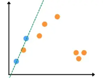
Random sample consensus, or RANSAC, is an iterative method for estimating a mathematical model from a data set that contains outliers. The RANSAC algorithm works by identifying the outliers in a data set and estimating the desired model using data that does not contain outliers. To understand better, let us assume that we have simple data with outliers and the best fitted-line using linear regression will be as follows.
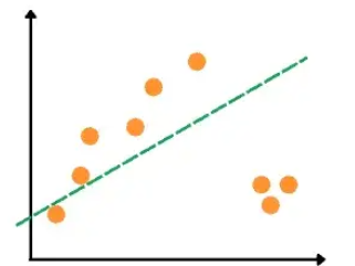
As you can see, because of an outlier, a linear regression line has been affected by it. If we apply the RANSAC algorithm to the same dataset, we will get the following best-fitted line.
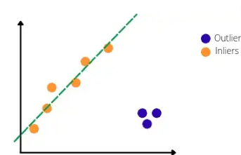
As you can see, the RANSAC model has detected the outlier and ignored it. Now let us understand step by step how the RANSAC algorithm detects and handles outliers.
How Does RANSAC Regression Detect Outliers?
An outlier is an observation that lies an abnormal distance from other values in a random sample from a population. They represent measurement errors, bad data collection, or show variables not considered when collecting the data. RANSAC algorithm trains the model by handling outliers. Let us understand how the RANSAC algorithm identifies outliers.
Basically, RANSAC is an iterative algorithm which means it will train the model on the given data over again and again. So, before start training the model, we have to specify the number of iterations. In this section, we will assume that we are training the RANSAC model with three iterations, and let us also assume that we have the following dataset.
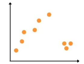
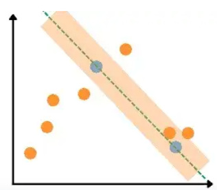
As our dataset is a two-dimensional dataset, the very first step in the training process of the RANSAC algorithm is that it will take any two random data points and will pass a line through them. In the case of the three-dimensional dataset, the algorithm will take three random points. In the next step, the algorithm will set a threshold value and every point that lies outside that threshold will be considered an outlier as shown below:
Now the algorithm has the best-fitted line in its first iteration. All the points in the threshold value will be considered inliers and the rest will be outliers. So, this will be the model for the first iteration and as we have three iterations, the process will again resume.
The algorithm will again take any two random data points, set a threshold value, and pass a line through them.
As you can see, we get the second best-fitted line as well. Now, the same process will be performed. Let us assume that the algorithm selects the following two data points this time.
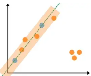
Once the algorithm will reach the maximum number of iterations, it will then select the best-fitted line ( a line with a maximum number of inliers) – in our case, the last one.
Handle Outliers in Regression Using the RANSAC Algorithm
Linear Regression is a machine learning algorithm based on supervised learning. It performs a regression task. Regression models a target prediction value based on independent variables. It is mostly used for finding out the relationship between variables and forecasting. We will use a linear regression model and at the same time will apply the RANSAC model to differentiate how the outliers can affect the model and how the RANSAC model trains the model without outliers.
First, let us import the dataset and get familiar with it.
# importin pandas module
import pandas as pd
# importing the dataset
dataset = pd.read_csv("DataForLR.csv")
# dataset heading
dataset.head()
Output:
Hours	Score
0	1.0	56
1	2.0	63
2	2.0	61
3	4.0	88
4	2.0	72
As you can see, we have two columns. Let us also visualize the dataset in a plot using matplotlib module.
# importing the module
import matplotlib.pyplot as plt
# plotting scattered plot
plt.scatter(dataset['Hours'], dataset['Score'] , c='m')
# labeling
plt.xlabel("Hours of study")
plt.ylabel("Overall marks")
plt.show()
Output:
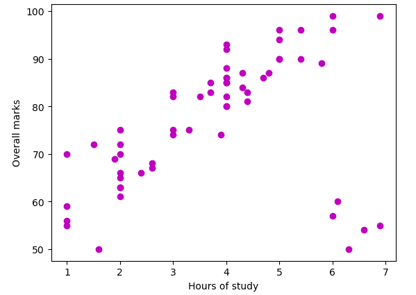
As you can see, we have visualized the data using a scattered plot.
Training the Linear Regression Model
Before training the linear regression model, let us first split the dataset into inputs and outputs.
# splitting dataset
x = dataset.iloc[:, :-1].values
y = dataset.iloc[:, 1].values
Now let us import the linear regression model and train the model using the given dataset.
# Importing linear regression form sklearn
from sklearn.linear_model import LinearRegression
# initializing the algorithm
regressor = LinearRegression()
# training linear regression model
regressor.fit(x,y)
As you can see, we have used all default parameter values to train the model. You can do hyperparameter tuning of linear regression to get the optimum model.
Once the training is complete, we will then visualize the model to see the best-fitted line.
# setting the size
plt.figure(figsize=(10, 6))
# ploting the dataset
plt.scatter(x, y, c='m' )
# ploting the testing dataset in line line
plt.plot(x, regressor.predict(x), color='green')
# labeling
plt.xlabel("Hours of study")
plt.ylabel("Overall marks")
plt.show()
Output:
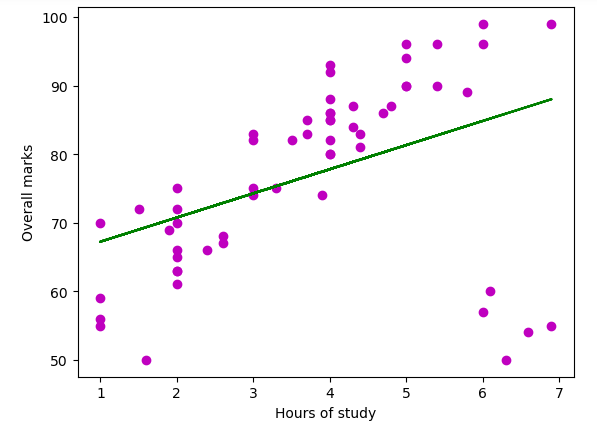
As you can see, we get the best-fitted line for the given dataset.
Training the RANSAC Model
Now let us train the RANSAC model on the same dataset. It will train the data on only inliers and will ignore the outliers. First, we will import the model and then train it on the training dataset.
# importing the module
from sklearn.linear_model import RANSACRegressor
# Initializing the model
ransac = RANSACRegressor()
# training the model
ransac.fit(x,y )
Once the training is complete, we will visualize the best-fitted line of the model.
# setting the size
plt.figure(figsize=(10, 6))
# ploting the dataset
plt.scatter(x, y, c='m' )
# ploting the testing dataset in line line
plt.plot(x, ransac.predict(x), color='red')
# labeling
plt.xlabel("Hours of study")
plt.ylabel("Overall marks")
plt.show()
Output:
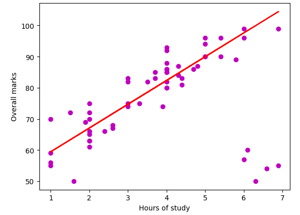
The regression line shown above is based on only inliers.
Compare Regression With Outliers and Without Outliers
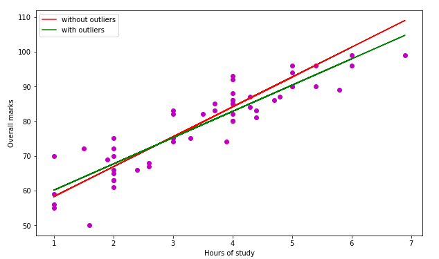
Now, we will compare both models and see how the regression line is different in both cases.
# setting the size
plt.figure(figsize=(10, 6))
# ploting the dataset
plt.scatter(x, y, c='m' )
# ploting the testing dataset in line line
plt.plot(x, ransac.predict(x), color='red', label='without outliers')
plt.plot(x, regressor.predict(x), color='green', label='with outliers')
# labeling
plt.xlabel("Hours of study")
plt.ylabel("Overall marks")
plt.legend()
plt.show()
Output:
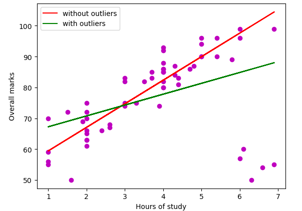
As you can see, the linear regression line is a little bit downward because of some outliers.
To understand clearly, let us predict the score of a student who studies 5 hours a day.
# input data
hours = [5]
# prediction of linear regression
p_regression = regressor.predict([hours])
# prediction of Ransac model
p_ransac = ransac.predict([hours])
# printing
print("With outliers :", p_regression)
print("\nWithout outliers: ", p_ransac)
Output:
With outliers : [90.35625396]
Without outliers:  [92.68064262]
As you can see, there is clearly a difference in the prediction because of the outliers in our dataset.
Number of Outliers in RANSAC
One of the important features of RANSAC is that we can also find the total number of outliers that have been detected in the dataset.
# importing the module
from sklearn.linear_model import RANSACRegressor
# Initializing the model
ransac = RANSACRegressor()
# training the model
ransac.fit(x,y )
# inlier mask
inlier_mask = ransac.inlier_mask_
print(inlier_mask)
Output:
[ True  True  True  True  True  True  True  True  True  True  True  True
  True  True  True  True  True  True  True  True  True  True  True  True
  True  True  True  True  True  True  True  True  True  True False  True
  True  True  True  True  True  True False  True  True  True  True  True
 False False  True  True  True False False False False False]
All the values that are False are the outliers that the algorithm has detected. You can manipulate the outliers on your own and visualize them using various visualization techniques in Python.
Summary
An iterative technique called Random Sample Consensus, or RANSAC, is used to estimate a mathematical model from a set of data that includes outliers. Using data that don’t contain outliers, the RANSAC algorithm calculates the required model after identifying the outliers in a data set. In this article, we discussed how we can handle outliers in a regression model using the RANSAC algorithm. Moreover, we also compared the results of linear regression with the RANSAC model.