Hyperparameter Tuning of XGBoost in Machine Learning

XGBoost is a type of Boosting algorithm that can be used for both regression and classification problems. Boosting algorithm creates a sequence of models instead of just one model and combines the predictions of all the models to come up with a strong predictive model. XGboost is an open-source supervised machine learning algorithm that creates a strong predictive model by combining various small and simple weak learners. In this article, we will discuss the XGBoost algorithm in detail and will implement it on various datasets including classification and regression datasets. Moreover, we will also learn how to do hyperparameter tuning of the XGboost algorithm by using various methods.

---

What is the XGBoost algorithm?

XGBoost is the short form of the eXtreme Gradient boosting algorithm. It is an open-source supervised machine learning. Some of the main features that make the XGBoost algorithm unique, fast, and more efficient are as follows

1. Cross-validation at each iteration: Cross-validation is a process in which the model is tested using different portions of the dataset in each iteration. The XGBoost algorithm has an internal parameter for the cross-validation and it tests each of the weak learners using the cross-validation method.
2. Parallel process: XGBoost uses OpenMP for parallel processing. But unlike random forests which create trees in parallel, the XGBoost creates individual trees using a parallel process.
3. Regularization: In Machines, learning regularization is a technique that is commonly used to reduce the risk of overfitting. Overfitting is when the models learn too many specific patterns about the training dataset and fail to generalize on the testing dataset. So, the XGBoost uses different regularization techniques in order to make sure that the model is not overfitted and that the findings can be generalized to the testing dataset.
4. Missing values: One of the essential features of the XGBoost algorithm is that it can handle the missing values automatically. That means we don’t need to handle missing values in the preprocessing step.
5. Tree pruning: Tree pruning is the process of removing the nodes from the trees that do not contribute to the classification.

So, these are some of the main features of the XGBoost algorithm that makes it one of the most popular boosting algorithms.

Steps in XGBoost Implementation

We will follow the following steps to implement the XGBoost algorithm on various datasets.

• Importing and exploring the dataset
• Splitting the dataset into the testing and training part
• Importing the XGBoost model
• Train the XGBoost model on the training dataset
• Use the testing dataset to evaluate the performance of the model
• Apply hyperparameter tuning if the model fails to perform well.

XGBoost Classifier Using Python

Now let us jump into the implementation part and use Python language to implement XGBoost on a classification dataset. For the sample, we will use the iris dataset as our classification dataset. Before going to the implementation part, make sure that you have installed the following Python modules on your system as we will be using them during the implementation part.

• xgboost
• sklearn
• pandas
• NumPy
• matplotlib
• seaborn

Let us first import the dataset.

Dataset
# importing the required modules
from sklearn import datasets
import pandas as pd
import numpy as np

# loading the iris dataset
dataset = datasets.load_iris()

# converting the data to DataFrame
data = pd.DataFrame(data= np.c_[dataset['data'], dataset['target']],
                     columns= dataset['feature_names'] + ['target'])

# printing the few rows
data.head()

Splitting the Dataset

Now, we will split the dataset into input variables and output variables.

input output
# splitting the dataset into input and output
Input = data.drop('target', axis=1)
Output =data['target']

Once, we have divided the dataset into the input and output variables, the next step is to split the dataset into the testing and training parts. We will also assign value 1 to the random state.

Splitting
# importing the module
from sklearn.model_selection import train_test_split

# splitting into testing and training parts
X_train, X_test, y_train, y_test = train_test_split(Input, Output, test_size=0.30, random_state=1)

Now it is time to import the XGBoost classifier and train the model.

Training the XGBoost Classifier

Now, we will use the XGBoost classifier to train on the classification dataset. We will use all the default parameter values.

XGBoost
# importing the xgboost module
import xgboost as xgb

# Default parameters
xgboost_clf = xgb.XGBClassifier()

# training the model
xgboost_clf.fit(X_train,y_train)

We have initialized the XGBoost classifier with all the default parameter values. We can check the values of these parameters by printing them.

Parameters
# printing default parameters values in XGBoost classifier
xgb.XGBClassifier().get_params()

Output:

{'objective': 'binary:logistic',
 'use_label_encoder': None,
 'base_score': None,
 'booster': None,
 'callbacks': None,
 'colsample_bylevel': None,
 'colsample_bynode': None,
 'colsample_bytree': None,
 'early_stopping_rounds': None,
 'enable_categorical': False,
 'eval_metric': None,
 'feature_types': None,
 'gamma': None,
 'gpu_id': None,
 'grow_policy': None,
 'importance_type': None,
 'interaction_constraints': None,
 'learning_rate': None,
 'max_bin': None,
 'max_cat_threshold': None,
 'max_cat_to_onehot': None,
 'max_delta_step': None,
 'max_depth': None,
 'max_leaves': None,
 'min_child_weight': None,
 'missing': nan,
 'monotone_constraints': None,
 'n_estimators': 100,
 'n_jobs': None,
 'num_parallel_tree': None,
 'predictor': None,
 'random_state': None,
 'reg_alpha': None,
 'reg_lambda': None,
 'sampling_method': None,
 'scale_pos_weight': None,
 'subsample': None,
 'tree_method': None,
 'validate_parameters': None,
 'verbosity': None}

These are all the default parameters on which the Xgboost model has been trained.

Evaluating the XGBoost Classifier

Once the training is complete, we can then use the testing dataset to make predictions using the XGBoost classifier.

predict
# testing the model
xgboost_preds = xgboost_clf.predict(X_test)

Now, we are not sure how accurate the model has made the predictions. So in order to know how well the predictions of the XGBoost classifier are, we will use different evaluation matrices to evaluate the performance of the model.

First, let us use the confusion matrix which will help us to visually see how many of the items have been classified incorrectly.

confusion matrix
# importing modules
import matplotlib.pyplot as plt
from sklearn.metrics import confusion_matrix, ConfusionMatrixDisplay

# confusion matrix plotting
cm = confusion_matrix(y_test,xgboost_preds, labels=xgboost_clf.classes_)

# labelling
disp = ConfusionMatrixDisplay(confusion_matrix=cm, display_labels=xgboost_clf.classes_)
disp.plot()
plt.show()

Output:

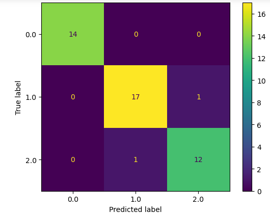
The XGBoost has performed exceptionally well using the default values of the parameters and only 2 of the output values have been classified incorrectly.

Let us also calculate the accuracy score of the model.

Accuracy
# importing the module
from sklearn.metrics import accuracy_score

# printing
print("The accuracy is: ", accuracy_score(y_test, xgboost_preds))

Output:

As you can see, we get an accuracy score of 95% which is pretty high.

XGBoost Regressor Using Python

Now, we will learn how we can use the XGBoost regressor to solve regression problems. In this section, we will be using a sample dataset about the price of houses. Let us first import the dataset and explore it a little bit.

dataset
# importing dataset 
data = pd.read_csv('house.csv')

# heading of the dataset
data.head()

Output:

The accuracy is:  0.9555555555555556

As you can see, the dataset contains some null values. We will not handle them as the XGBoost algorithm can automatically handle Null values.

XGBoost Regressor

Now, we will use a very simple dataset that contains various features about the house and the target column is the price of the house. We will implement an XGBoost regressor model in this case which will help us create a model to predict the price of the house.

First we will split the data into input and output values, after importing the data.

Input output
# input and output variables
Input = data.drop('price', axis=1)
Output = data.price

Next, we have to split the dataset into the testing and training parts so that we can train the model and then use the testing data to evaluate the model.

Splitting
# splitting into testing and training parts
X_train, X_test, y_train, y_test = train_test_split(Input, Output, test_size=0.25)

Now, our dataset is ready and can be used to train the model.

Training the XGBoost Regressor

Let us now import the XGBoost regressor and then train the model using the training dataset.

Fitting model
# xgboost regressor
model = xgb.XGBRegressor()

# training the model
model.fit(X_train,y_train)

Once the training is complete, we can then use the testing data to make predictions.

Prediction
# making predictions
model_pred = model.predict(X_test)

As you can see, the model has made predictions, but we are not sure how accurate these predictions are. So, let us evaluate the performance of the model

Evaluate the XGBoost Regressor

Let us first visualize the actual and the predicted values of the model to see how close they are.

Plotting
# figure size
plt.figure(figsize=(12, 8))

# acutal values
plt.plot([i for i in range(len(y_test))],y_test, label="actual values")

# predicted values
plt.plot([i for i in range(len(y_test))],model_pred, c='m',label="predicted values")
plt.legend()
plt.show()

Output:

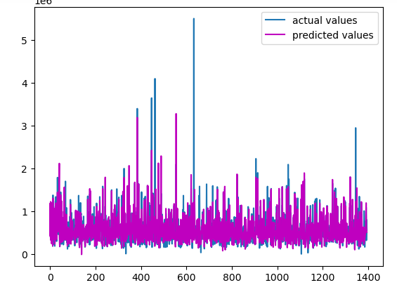
As you can see, the predictions are pretty much close to the actual values.

Let us also calculate the R-square score of the model as well.

r2 score
#importing the r-square score
from sklearn.metrics import r2_score

# calculating the r score 
print('R score is :', r2_score(y_test, model_pred))

Output:

R score is : 0.6125213393080935

We got a really good R-square score which means the predictions were close to the actual values.

Hyperparameter Tuning of XGBoost Algorithm

As we know many important parameters in XGBoost directly affect the performance of the model. In the above sections, we have used all the default values of these parameters but changing the values of these parameters can directly affect the performance of the model. In this section, we will learn how to find the optimum values for these parameters using Hyperparameter tuning of XGBoost to get an optimum result.

Make sure that you have installed the following modules as we will be using them in the hyperparameter tuning.

Importing modules
# importing  modules for Hyperparameter tuning of XGBoost
from numpy import mean
from sklearn.datasets import make_classification
from sklearn.model_selection import cross_val_score
from sklearn.model_selection import RepeatedStratifiedKFold
from matplotlib import pyplot
from sklearn.tree import DecisionTreeClassifier
from sklearn.model_selection import GridSearchCV
from numpy import arange

Let us first import the dataset and split it.

dataset
# loading the iris dataset
dataset = datasets.load_iris()

# converting the data to DataFrame
data = pd.DataFrame(data= np.c_[dataset['data'], dataset['target']],
                     columns= dataset['feature_names'] + ['target'])


# splitting the dataset into input and output
Input = data.drop('target', axis=1)
Output =data['target']

Once, we import the dataset, the next step is to create a function that will evaluate the performance of the model based on the accuracy score.

Function
# function for the validation of model
def evaluate_model(model, Input, Ouput):
    
    # defining the method of validation
    cv = RepeatedStratifiedKFold(n_splits=10, n_repeats=3)
    
    
    # validating the model based on the accurasy score
    accuracy = cross_val_score(model, Input, Ouput, scoring='accuracy', cv=cv, n_jobs=-1)
    
#     returning the accuracy score
    return accuracy

Now, let us create different functions for each of the parameters and then use different values to find the optimum value.

Finding the Optimum Number of Iterations Using Hyperparameter Tuning of XGBoost

Let us now create a function that will return multiple models, each having different interaction values.

classifier
# fuction to create models
def build_models():
    
#     dic of models
    models = dict()
    
    # number of decision stumps
    decision_stump= [10, 50, 100, 500, 1000]
        
#    using for loop to iterate though trees
    for i in decision_stump:
        
#         building model with specified trees
        models[str(i)] = xgb.XGBClassifier(n_estimators=i)
    
#     returning the model
    return models

This function returns a dictionary of different XGBoost models with a different number of iterations. Let us now call this and the evaluation function to get the optimum number of iterations.

Iteration
# calling the build_models function
models = build_models()

# creating list
results, names = list(), list()

# using for loop to iterate thoug the models
for name, model in models.items():
    
    # calling the validation function
    accuracy = evaluate_model(model, Input, Output)
    
    
    # appending the accuray socres in results
    results.append(accuracy)
    names.append(name)
    
    
    # printing -Hyperparameter tuning of XGBoost
    print('---->Iterations (%s)---Accuracy( %.5f)' % (name, mean(accuracy)))

Output:

---->Iterations (10)---Accuracy( 0.96222)
---->Iterations (50)---Accuracy( 0.94444)
---->Iterations (100)---Accuracy( 0.94889)
---->Iterations (500)---Accuracy( 0.94667)
---->Iterations (1000)---Accuracy( 0.94667)

As you can see, we get an optimum result for 10 iterations. Let us also visualize the same results using a boxplot.

box plot
# plotting box plot of the 
plt.boxplot(results, labels=names,showmeans=True)

# showing the plot
plt.show()

Output:

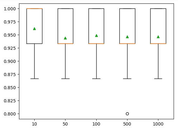
The boxplots also showed that the model has the highest accuracy when the number of iterations are 10.

Finding the Optimum Number of Features Using Hyperparameter Tuning of XGBoost

Features are simply the input variables. Sometimes, our dataset contains a large number of input features and it becomes hard to find the optimum number of features that contribute most to the output. In this section, we will learn how we can find the optimum number of features in the XGBoost algorithm.

Let us first create a function that will return a dictionary of models having a different number of features.

Function
# creating the function 
def build_models():
    
#     creating dic of models
    models = dict()
    
    # explore features numbers from 1-4
    for i in range(1,5):
        
#         appending the models
        models[str(i)] = xgb.XGBClassifier(max_features=i)
    
#     returining the models
    return models

Once, we create the model for a different number of features, we can then call this function and evaluation function which will help us which model has the highest accuracy.

Model
# calling the function
models = build_models()

# creating the list
results, names = list(), list()

# for loop to iterate through the models
for name, model in models.items():
    
    
    # calling the evaluting function
    accuracy = evaluate_model(model, Input, Output)
    
#     storing the accurcy
    results.append(accuracy)
    names.append(name)
    
#     printing - Hyperparameter tuning of XGBoost
    print('---->Features(%s)---Accuracy( %.5f)' % (name, mean(accuracy)))

Output:

---->Features(1)---Accuracy( 0.95333)
---->Features(2)---Accuracy( 0.94667)
---->Features(3)---Accuracy( 0.96667)
---->Features(4)---Accuracy( 0.94667)

As you can see the optimum accuracy is when we use 3 features at the same time. Now, you can also visualize the features using the box plot as we did before.

Finding the Optimum Sample Size Using Hyperparameter Tuning of XGBoost

We can also change the sample size to be used to train each weak learner in the XGBoost algorithm. Let us create a function that will return multiple models with different sample sizes.

Model function
# creating the function
def build_models():
    
#     dic of models
    models = dict()
    
#     exploring different sample values
    for i in arange(0.1, 1.1, 0.1):
        
#         key value
        k = '%.1f' % i
    
#     appending the model
        models[k] = xgb.XGBClassifier(subsample=i)
    return models

Now, we will call the above function and the evaluation function which will help us to find the optimum size of sample data.

Samples
# calling the function
models = build_models()
# creating the list
results, names = list(), list()
# for loop to iterate through the models
for name, model in models.items():
    
    
    # calling the evaluting function
    accuracy = evaluate_model(model, Input, Output)
    
#     storing the accurcy
    results.append(accuracy)
    names.append(name)
    
#     printing - Hyperparameter tuning of XGBoost
    print('Samples(%s)---Accuracy( %.5f)' % (name, mean(accuracy)))

Output

Samples(0.1)---Accuracy( 0.94889)
Samples(0.2)---Accuracy( 0.95111)
Samples(0.3)---Accuracy( 0.94000)
Samples(0.4)---Accuracy( 0.94000)
Samples(0.5)---Accuracy( 0.95111)
Samples(0.6)---Accuracy( 0.94444)
Samples(0.7)---Accuracy( 0.95111)
Samples(0.8)---Accuracy( 0.94889)
Samples(0.9)---Accuracy( 0.94667)
Samples(1.0)---Accuracy( 0.95111)

As you can see, we get the highest accuracy when the sample size is 0.9.

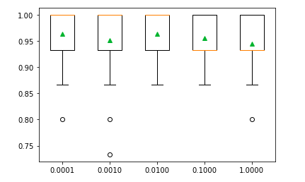
Finding Optimum Learning Rate Using Hyperparameter Tuning of XGBoost

The learning rate is the weight used to train the model in each of the iterations. We can use various values for the learning rate. Let us first create a function that returns a dictionary of models with different learning rates.

function
# creating function
def build_models():
    
#     creating dic of models
    models = dict()
    
#     different learning rates
    for i in [0.0001, 0.001, 0.01, 0.1, 1.0]:
        
#         key value
        k = '%.4f' % i
    
#     appending the models
        models[k] = xgb.XGBClassifier(learning_rate=i)
    return models

Let us now call the above function and the evaluation function that will help us to find the optimum value of the learning rate.

Learning rate
# calling the function
models = build_models()
# creating the list
results, names = list(), list()
# for loop to iterate through the models
for name, model in models.items():
    
    
    # calling the evaluting function
    accuracy = evaluate_model(model, Input, Output)
    
#     storing the accurcy
    results.append(accuracy)
    names.append(name)
    
#     printing - Hyperparameter tuning of XGBoost
    print('Learning Rate(%s)---Accuracy( %.5f)' % (name, mean(accuracy)))

Output:

Learning Rate(0.0001)---Accuracy( 0.96000)
Learning Rate(0.0010)---Accuracy( 0.95111)
Learning Rate(0.0100)---Accuracy( 0.95778)
Learning Rate(0.1000)---Accuracy( 0.95333)
Learning Rate(1.0000)---Accuracy( 0.95111)

As you can see, we get the highest accuracy value for a learning rate of 0.01.

Finding the Optimum Depth Using Hyperparameter Tuning of XGBoost

As we know the depth of the decision tree ( used as a weak learner in XGBoost) impacts the overall outcome of the XGBoost algorithm. Let us create a function that will return different models with different depths of decision trees.

Function
# building function for the model
def build_models():
    
#     creating dic of models
    models = dict()
    
#     specifying the depth of trees
    for i in range(1,12):
        
#         appending the models
        models[str(i)] = xgb.XGBClassifier(max_depth=i)
        
#   returining the model
    return models

Now let us call the evaluation function which will help us to find the optimum depth of the trees.

Depth of tree
# calling the function
models = build_models()

# creating lists 
results, names = list(), list()

# iterating through the models
for name, model in models.items():
    
    # calling the evalution function
    accuracy = evaluate_model(model, Input, Output)
    
    # appending the results
    results.append(accuracy)
    names.append(name)
    
#     printing - Hyperparameter tuning of XGBoost
    print('Decision tree depth (%s)---Accuracy( %.5f)' % (name, mean(accuracy)))

Output:

Decision tree depth (1)---Accuracy( 0.94000)
Decision tree depth (2)---Accuracy( 0.94444)
Decision tree depth (3)---Accuracy( 0.94000)
Decision tree depth (4)---Accuracy( 0.94889)
Decision tree depth (5)---Accuracy( 0.95111)
Decision tree depth (6)---Accuracy( 0.95333)
Decision tree depth (7)---Accuracy( 0.94444)
Decision tree depth (8)---Accuracy( 0.95111)
Decision tree depth (9)---Accuracy( 0.94222)
Decision tree depth (10)---Accuracy( 0.95111)
Decision tree depth (11)---Accuracy( 0.94667)

As you can see, we get the highest accuracy when the depth of the tree is 6 and 9.

GridSearchCV for Hyperparameter Tuning of XGBoost

GridSearchCV is a process of finding optimum values for various parameters from the given range.

Let us first initialize the model and then specify the values for different parameters.

XGBclassifier
# defiing the model
model = xgb.XGBClassifier()


# creating a dict of grids
grid = dict()

# values for iteration
grid['n_estimators'] = [10, 50, 100, 500]

# values for learning rate
grid['learning_rate'] = [0.0001, 0.001, 0.01, 0.1, 1.0]

# values for the sampel
grid['subsample'] = [0.5, 0.7, 1.0]

# values for teh depth of tree
grid['max_depth'] = [3, 4, 5]

Let us now use the GridSearchCV to find the optimum values for the parameters from the above ranges.

GridsearchCV
# defining the cv
cv = RepeatedStratifiedKFold(n_splits=10, n_repeats=3)


# applying the gridsearchcv method
grid_search = GridSearchCV(estimator=model, param_grid=grid, n_jobs=-1, cv=cv, scoring='accuracy')

# storing the values
grid_result = grid_search.fit(Input, Output)


# printing the best parameters - Hyperparameter tuning of XGBoost
print("Accuracy score: %f using %s" % (grid_result.best_score_, grid_result.best_params_))

Output:

Accuracy score: 0.966667 using {'learning_rate': 0.0001, 'max_depth': 4, 'n_estimators': 100, 'subsample': 0.7}

The GridSearchCV returns the optimum values for the parameters.

NOTE: You can get access to the source code and the dataset used in this article from my GitHub account. Don’t forget to follow and give me a star.

Summary

XGBoost is a supervised boosting learning algorithm that can be used for regression and classification problems. Similar to other boosting algorithms, the XGBoost algorithm trains various weak learners and combines them to come up with a strong predictive model. Unlike many other boosting algorithms, the XGboost algorithm can handle Null values automatically. In this article, we learned how the XGBoost algorithm works and find the optimum parameter values using various methods for Hyperparameter tuning of XGBoost.

Frequently Asked Questions

What is the XGboost algorithm?

XGBoost is a supervised boosting learning algorithm that can be used for regression and classification problems. Similar to other boosting algorithms, the XGBoost algorithm trains various weak learners and combines them to come up with a strong predictive model

How to use XGBoost in Python?

First, install the XGboost on your system and then initialize the model. You can train the model using the training dataset and then use the testing dataset to test the performance of the model.

How to install XGboost?

Similar to any other Python modules, XGBoost can be installed on your system using the pip command.