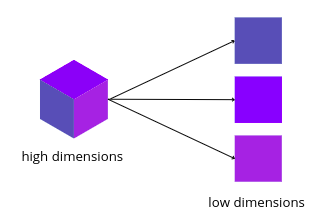
Principal component analysis in Python (PCA) is one of the best and simplest techniques for dimensionality reduction. Dimensionality reduction is simply the transfer of data from high dimensions to low dimensions by retaining all the important attributes and features. The PCA algorithms transform the highly correlated attributes into simple linear uncorrelated ones. In this article, we will discuss how the principal component analysis (PCA) converts high-dimensional data into low-dimensional ones and we will implement PCA using Python on a sample dataset. Moreover, we will learn how we can use principal component analysis (PCA) to reduce the size of an image.
You may also like to visit Python for Machine Learning.
What is the Principal Component Analysis in Python?
The principal component analysis is an unsupervised machine learning algorithm that converts highly correlated attributes to linear uncorrelated attributes. A dataset having a lot of attributes may be different to analyze and may also lead to overfitting of the machine learning models. So, to solve such an issue, we use principal component analysis that converts high dimensionality into a low dimensionality dataset.
Example of Principal Component Analysis (PCA)
Now, let us understand the dimensional reduction of the principal component analysis (PCA) using an example. Let us say we have the dataset that contains the obtained scores of 4 students in two subjects as shown below:
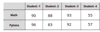
As you can see, we have scores of 4 students in the ML subject. We can easily visualize this dataset using a simple number line or bar chart.
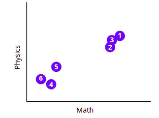
We can plot the data set of students’ obtained marks in various different plots because it has fewer dimensions. The problem arises when we have a dataset of more than 3 subjects because we can only plot data in 3 dimensions. For example, let us say we have the following dataset.
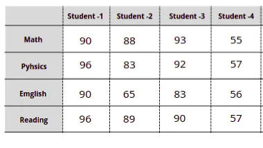
Now, we cannot plot one graph representing all these data because then the plot will be 4 dimensional. Here comes the PCA to help us plot such datasets in 2-D or 3-D by reducing the dimensional.
Principal Component Analysis in Python Using Sklearn
Now, we will Python and sklearn modules to implement the PCA on the sample dataset. The dataset is about house pricing in Dushanbe city. The input variables are the number of rooms, floors, area, and location of the house. Before going to the implementation part, make sure that you have installed the following modules as we will be using them in the implementation part.
- sklearn
- NumPy
- pandas
- matplotlib
- plotly
- seaborn
- opencv-python
You can use the pip command to install these modules on your system.
Getting Familiar with the Dataset
We will use pandas to import the dataset and explore it as pandas is a very useful and powerful Python module for exploring datasets.
Let us import the dataset and print out a few rows.
# importing the pandas module
import pandas as pd

# importing the dataset
data = pd.read_csv('house.csv')

# printing the heading
data.head()
We have null values as well. We will use the dropna() method to drop the null values from the dataset.
# droping the null values
data.dropna(axis=0, inplace=True)

# verifying if still there are null values
data.isnull().sum()
There are no null values this time. We will also drop the output values from the dataset as we don’t need them for dimensional reductions.
Implementing Principal Component Analysis in Python
Now, we will use the sklearn module in Python to build a PCA model which will help us reduce the dataset’s dimensions.
Let us first import the module and initialize the model.
# importing the principal component analysis in Python
from sklearn.decomposition import PCA

# principal component analysis in Python
pca = PCA()
Now let us list all the attributes and then train the PCA model on the dataset.
# listing all the attributes
features = ['number_of_rooms','floor','area','latitude','longitude']

# Training the principal component analysis in Python
PCA_components = pca.fit_transform(data[features])
Once, the training is complete, we can then visualize the PCAs.
# importing the module
import plotly.express as px


# plot labeling
labels = {str(i): f"PC {i+1} ({var:.1f}%)"
    for i, var in enumerate(pca.explained_variance_ratio_ * 100)}

# Ploting the scattered graph
fig = px.scatter_matrix(PCA_components,labels=labels,dimensions=range(4))

# visualizing the plot
fig.update_traces(diagonal_visible=False)
fig.show()
Output:
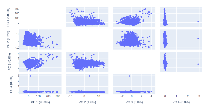
As you can see, PCA1 and PCA2 have the highest variance. That means we can exclude PCA3 and PCA4 to visualize the same data in 3d and 2d plots.
Principal Component Analysis to Reduce Dimensions to 3D
Now, we will train the PCA model again with only 3 PCAs so that we can easily visualize the data without losing any important features.
# initializing the PCA with 3 components
pca = PCA(n_components=3)

# Training principal component analysis in Python
PCA_3components = pca.fit_transform(data[features])
Once, the training is complete, the PCA will reduce the dimensions of the dataset to 3 so that we can easily visualize it.
# calculating the total variance
total_var = pca.explained_variance_ratio_.sum() * 100

# creating 3-d graph
fig = px.scatter_3d(
    PCA_3components, x=0, y=1, z=2,
    title=f'Total Variance: {total_var:.2f}%',
    labels={'0': 'PC 1', '1': 'PC 2', '2': 'PC 3'}
)

# showing the plot
fig.show()
Output:
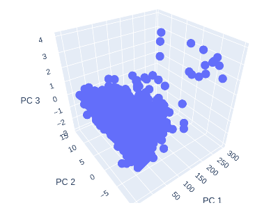
We were able to plot the complex dataset in 3D with the help of PCA modeling.
Principal Component Analysis in Python to Reduce Dimensions to 2D
We can further decrease the dimensions of the dataset to 2 dimensions as well. Let us again train the model with 2 PCA components.
# initializing the PCA with 2 components
pca = PCA(n_components=2)

# Training principal component analysis in Python
PCA_2components = pca.fit_transform(data[features])
Once the training of the principal component analysis model on 2 components is finished, we can then plot the components on the 2-dimensional graph.
# Ploting the PCA in 2 D
fig = px.scatter(PCA_2components, x=0, y=1)
fig.show()
Output:
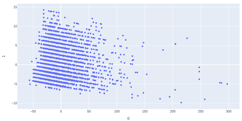
We have successfully plotted the 2D plot of the dataset using PCA.
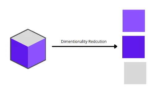
Principal Component Analysis (PCA) to Reduce the Image Size
One of the real-life applications of PCA is to reduce the size of an image. Sometimes, in machine learning, while training the model if the size of the images is too large then it can take a lot of time. So, in order to reduce the training time, we can use PCA to compress the size of the images.
In this section, we will learn how we can use principal component analysis to reduce the size of an image. First, let us open the original image using open-cv Python and matplotlib modules.
# importing the opencv python and maplotlib
import cv2
import matplotlib.pyplot as plt

# reading the image
img = cv2.cvtColor(cv2.imread('PCA.png'), cv2.COLOR_BGR2RGB)

# plotting the image using matplotlib
plt.imshow(img)
plt.show()
Output:

We have plotted the image. Now, we will apply various methods and functions to explore this image.
Splitting the Image in RGB
As we know that this image is RGB(colored image). We can also verify it by printing the shape of the image.
# printing the shape
img.shape
Output:
(256, 496, 3)
As you can see, the size of the image is 356×496 and the 3 means it is a colored image. we can separate these three layers ( Red, green, and blue) of the image and visualize them separately.
#Splitting different layers of the image
blue,green,red = cv2.split(img)


# fixing the size of image
fig = plt.figure(figsize = (12, 6))

# plotting blue color
fig.add_subplot(131)

# adding the title
plt.title("Blue Layer")
plt.imshow(blue)

# plotting green color
fig.add_subplot(132)

# adding the title
plt.title("Green Layer")
plt.imshow(green)

# plotting the red color
fig.add_subplot(133)

# adding the title
plt.title("Red Layer")
plt.imshow(red)
plt.show()
Output:
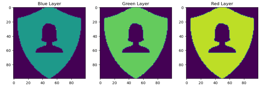
The images have been separated into different colors. Now, if we check the shape of each image, there will be no more RGB images.
# printing the shape
print(red.shape)
print(green.shape)
print(blue.shape)
Output:
(365, 496)
(365, 496)
(365, 496)
Now in the shape, there is no third value that represents the colored images.
Reducing the Size of the Image Using PCA
Now, we will practically apply the principal component analysis to the image to reduce the size of the image.
First, let us scale the three images ( layers) in a range of 0 to 1 by dividing each value by 255.
# scalling the images
blue_img = blue/255
green_img = green/255
red_img = red/255
Now, we will apply the principal component analysis to each of the layers of the image and will reduce the size to 40 components.
# Reducing size with 40 components
pca = PCA(n_components=40)

# training on the  blue layer
pca.fit(blue_img)

# trainsforming the blue layer
trans_pca_b = pca.transform(blue_img)

# training on the  green layer
pca.fit(green_img)

# trainsforming the green layer
trans_pca_g = pca.transform(green_img)


# training on the  red layer
pca.fit(red_img)

# trainsforming the red layer
trans_pca_r = pca.transform(red_img)
Now, each layer of the image has been reduced. To verify the compression of the image, we will again print out the shapes of the images.
# shape of reduced images
print(trans_pca_b.shape)
print(trans_pca_r.shape)
print(trans_pca_g.shape)
Output:
(356, 40)
(356, 40)
(356, 40)
As you can see, the size of the image has been reduced to only 40 components as defined.
Visualizing the Reduced Image Using PCA
As you have seen, we were able to use the principal component analysis algorithm to decrease the size of the image to 40 components. It is time to transform each layer back to the image.
# transforming back principal component analysis in Python
blue_arr = pca.inverse_transform(trans_pca_b)
green_arr = pca.inverse_transform(trans_pca_g)
red_arr = pca.inverse_transform(trans_pca_r)
Once the transformation is complete, then we will merge the layers back to again form an RGB image.
# merging to form RGB image
img_reduced= (cv2.merge((blue_arr, green_arr, red_arr)))
NOTE: You can access the source code and dataset from my GitHub account. Don’t forget to give it a star and follow.
Summary
The principal component analysis is an unsupervised method to reduce the dimensions of the dataset. It is mostly used in the preprocessing part of the data to get only the important features of the dataset. Moreover, it has high applications in image compression as well. In this article, we discussed how the PCA is working and implemented it into a sample dataset to reduce the attributes. Furthermore, we will use PCA to reduce the size of an image.