
Are you looking for an in-depth article about image processing using TensorFlow? Well, let’s learn in-depth image processing with neural networks using TensorFlow.
One of the tasks that deep neural networks (DNNs) excel at is image recognition. Computer programs called neural networks are made to spot patterns in the dataset. They are made up of input, hidden layers, and output layers. Image processing in the neural network is simply using neural networks for image processing. In this article, we will learn about image processing using TensorFlow. Mainly, we will learn how we can use TensorFlow Module to crop, filter, and rotate images.
What is Image Processing?
Image processing using TensorFlow is a technique for applying various procedures to an image in order to improve it or extract some relevant information from it. It is a kind of signal processing where the input is an image and the output can either be another image or features or characteristics related to that image. Image processing is one of the technologies that is currently expanding quickly.
There are basically the main steps involved in image processing using TensorFlow.
- Importing images using any tool
- applying different image processing techniques
- Output processed image
Also, there are two main types of image processing.
- Analogue image processing: This method is applied to the hard copies of images.
- Digital image processing: As the name suggests, digital image processing is the processing of images using computers in digital form. In this article, we will be using digital image processing using TensorFlow
What are Convolutional Neural Networks (CNN) in TensorFlow?
Convolutional neural networks are Neural networks that are commonly used to detect patterns in images. They can e used on any type of image ( binary, grayscale, or colored). Similar to any other Neural network, CNN is also composed of the input layer, hidden layers, and an output layer. But unlike other Neural networks, CNN needs to perform additional operations on the images before feeding the to CNN. Some of those preprocessing steps are:
- Filtering
- pooling
- padding
- flattening
The full architecture of CNN looks like this:
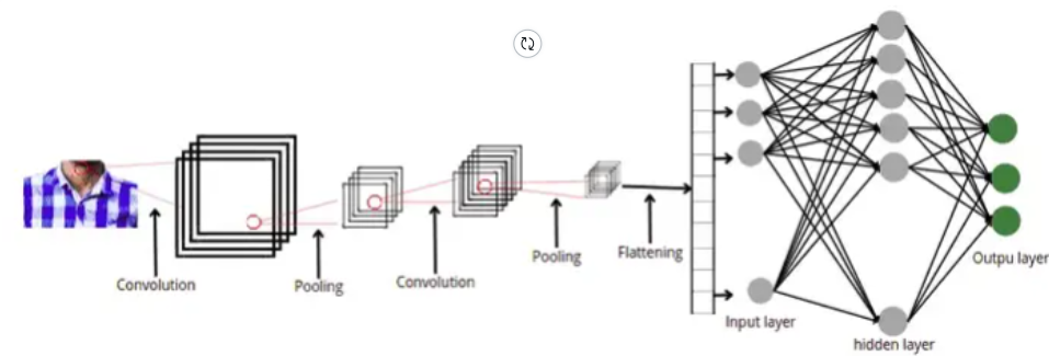
As you can see, there are a few steps of preprocessing images before feeding them to the neural networks.
Why CNN is used in Image Processing?
As we already discussed various preprocessing methods can be applied to the images before feeding them to the neural network. So, these processes are image processing. We can reduce the size, apply filters, rotate images, or increase contrast levels by using CNN.
To deal with images in Machine Learning, we need to first extract the pixel values and bring the image in numeric form. Then we can perform different kinds of operations on the image array. But in case of CNN, we just use the image, and the conversion is done automatically for us.
Image Processing Using TensorFlow
Now, let us dive directly into the practical part and start the image processing using TensorFlow. We will use a sample image in this case. You can get access to the data and the source code from my GitHub account.
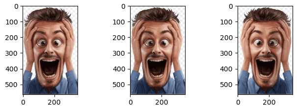
Let us first open the image and see the original image, before applying any of the image processing methods.
# importing the required modules
import matplotlib.pyplot as plt
import matplotlib.image as mpimg
# importing the image
image = mpimg.imread('Profile.png')
# showing the image
plt.imshow(image)
plt.show()
Output:
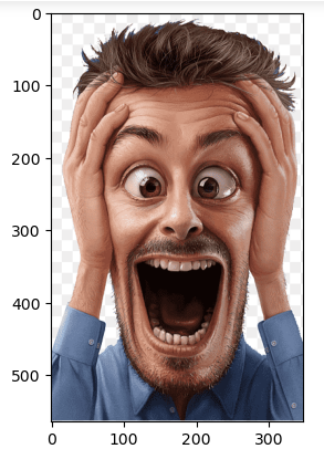
We will apply different image processing methods to the above image.
Detecting Edges of the Image Using TensorFlow
Now we will use the TensorFlow module to detect the edges of the above image using the Sobel edge-detecting method. Before detecting edges, we need to define the filters that will help us in detecting the edges.
#image processing with neural networks
#importing the module
import numpy as np
# sobel 3x3 filter - horizonal edges
sobel_y = np.array([[ -1, -2, -1],
                   [ 0, 0, 0],
                   [ 1, 2, 1]])

#  3X3 filter -- vertical edge detection
sobel_x = np.array([[-1, 0, 1],
                   [-2, 0, 2],
                   [-1, 0, 1]])
Now, let us apply these filters to detect the horizontal and vertical edges in the image.
# importing the module for image processing using tensorflow
import cv2
# Convert to grayscale for filtering
gray = cv2.cvtColor(image, cv2.COLOR_RGB2GRAY)
# filter the image using filter
filtered_image1 = cv2.filter2D(gray, -1, sobel_y)
filtered_image2 = cv2.filter2D(gray, -1, sobel_x)
# plotting the filtered images
f, ax = plt.subplots(1, 2, figsize=(16, 4))
# plotting the horizontal edge detections
ax[0].set_title('horizontal edge detection')
ax[0].imshow(filtered_image1, cmap='gray')
# plotting the vertical edge dections
ax[1].set_title('vertical edge detection')
ax[1].imshow(filtered_image2, cmap='gray')
Output:
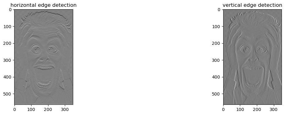
As you can see, we were able to detect the edges in the image.
Visualizing Feature Paps in Image Processing Using TensorFlow
When filters are applied to the input, such as the input image or another feature map to capture the results is known as feature maps. The goal of the feature map is to understand the main features of the input image.
The Keras Framework contains a pre-trained model that we will be using. There are several CNN models available, but we’ll choose the VGG model. Due to its depth (16 learned layers) and excellent performance, the filters and feature maps that arise will catch useful features.
Let us first import the VGG model and then initialize it.
# importing the modules for image processing using tensorflow
from tensorflow.keras.applications.vgg16 import VGG16
from tensorflow.keras.models import Model
#initializing the model
model = VGG16()
The next step is to know the shape of the input images in each of the layers of the model so that we can use an appropriate size.
# image processing using tensorflow
# looping the layers
for i in range(len(model.layers)):

#     checiking for each layer
    layer = model.layers[i]
    if 'conv' not in layer.name:
        continue

#     printing the output
    print(i , layer.name , layer.output.shape)
Output:
1 block1_conv1 (None, 224, 224, 64)
2 block1_conv2 (None, 224, 224, 64)
4 block2_conv1 (None, 112, 112, 128)
5 block2_conv2 (None, 112, 112, 128)
7 block3_conv1 (None, 56, 56, 256)
8 block3_conv2 (None, 56, 56, 256)
9 block3_conv3 (None, 56, 56, 256)
11 block4_conv1 (None, 28, 28, 512)
12 block4_conv2 (None, 28, 28, 512)
13 block4_conv3 (None, 28, 28, 512)
15 block5_conv1 (None, 14, 14, 512)
16 block5_conv2 (None, 14, 14, 512)
17 block5_conv3 (None, 14, 14, 512)
So now, based on the above information we can build a new model that takes the image size of any of the above-mentioned sizes along with their respective layers.
# creating a new model with size 224 224
model = Model(inputs=model.inputs , outputs=model.layers[1].output)
Now, our model is ready so let us import the image and convert it to numeric values.
# importing the required modules for image processing using tensorflow
from tensorflow.keras.preprocessing.image import load_img
from tensorflow.keras.preprocessing.image import img_to_array
from numpy import expand_dims
# importing the image and specifying the output size
image = load_img("Profile.png" , target_size=(224,224))
# convert the image to an array
image = img_to_array(image)
# expand dimensions so that it represents a single 'sample'
image = expand_dims(image, axis=0)
As we have pixel value, so let us scale them properly.
# importing the module
from tensorflow.keras.applications.vgg16 import preprocess_input
# scaling pixel values
image = preprocess_input(image)
Now it is time to visualize the feature map of the image.
# importing the module
from matplotlib import pyplot
#calculating features_map
features = model.predict(image)
# plotting the size
fig = pyplot.figure(figsize=(20,15))
# looping though each feature
for i in range(1,features.shape[3]+1):

#     plotting gray scale image
    pyplot.subplot(8,8,i)
    pyplot.imshow(features[0,:,:,i-1] , cmap='gray')

pyplot.show()
Output:
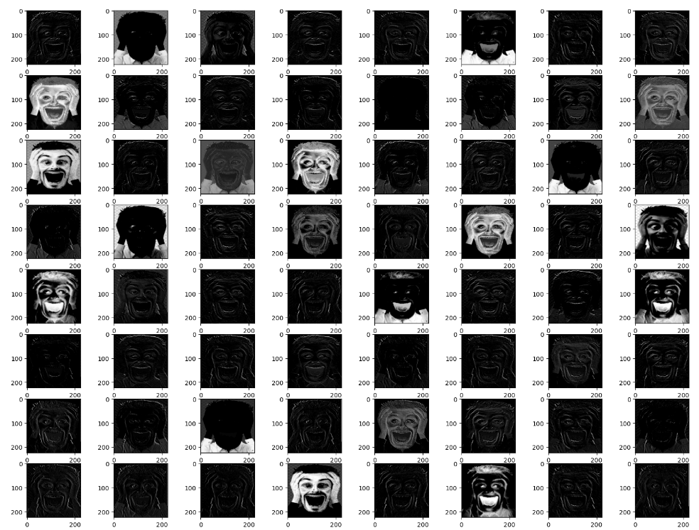
In a similar way, we can also visualize the feature maps in other layers as well.
# defining new model
model2 = VGG16()
# listing the layers to be displayed
blocks = [ 3, 5 , 10 , 15 , 17]
outputs = [model2.layers[i].output for i in blocks]
# creating the model and predicting
model2 = Model( inputs= model2.inputs, outputs = outputs)
feature_map = model2.predict(image)
# looping over the feature map and ploting
for i,fmap in zip(blocks,feature_map):
    fig = pyplot.figure(figsize=(20,15))

#     visualizing with block number
    fig.suptitle("BLOCK_{}".format(i) , fontsize=20)
    for i in range(1,features.shape[3]+1):
        pyplot.subplot(8,8,i)
        pyplot.imshow(fmap[0,:,:,i-1] , cmap='gray')

pyplot.show()
Output:
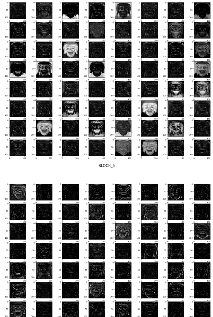
As you can see, we have visualized the feature map in different layers.
Flipping the Image in TensorFlow
We will now use the TensorFlow module for the flipping of the image. We can flit horizontally and vertically. First, we will learn how we can flip the image horizontally.
First, we will import the modules and the image and will convert them into a NumPy array as we did earlier.
# importing the module
from tensorflow.keras.preprocessing.image import ImageDataGenerator
# loading the image
image = load_img('Profile.png')
# coverting the image to array
dataImage = img_to_array(image)
Let us now flip the image horizontally and show the effect.
# expending the dimensions
imageNew = expand_dims(dataImage, 0)
# flipping horizontally
imageDataGen = ImageDataGenerator(horizontal_flip=True)
# applying the transfromation on the image
iterator = imageDataGen.flow(imageNew, batch_size=1)
plt.figure(figsize=(8, 8))
# using for loop to iterate and visualize
for i in range(3):

	# showing subplots
	pyplot.subplot(330 + 1 + i)

	# generating images of each batch
	batch = iterator.next()
	image = batch[0].astype('uint8')
	plt.imshow(image)
plt.show()
Output:
Let us also apply vertical flipping to the above image.
# flipping horizontally
imageDataGen = ImageDataGenerator(vertical_flip=True)
# applying the transfromation on the image
iterator = imageDataGen.flow(imageNew, batch_size=1)
plt.figure(figsize=(8, 8))
# using for loop to iterate and visualize
for i in range(3):

	# showing subplots
	pyplot.subplot(330 + 1 + i)

	# generating images of each batch
	batch = iterator.next()
	image = batch[0].astype('uint8')
	plt.imshow(image)
plt.show()
Output:
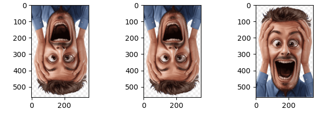
As you can see, we have successfully flipped the image vertically and horizontally.
Randomly Adjusting Brightness of Image Using TensorFlow
The brightness of the image can be adjusted by increasing the darkness or brightness.
# expand dimension to one sample
samples = expand_dims(dataImage, 0)
# create image data augmentation generator
datagen = ImageDataGenerator(brightness_range=[0.2,1.0])
# iterations
it = datagen.flow(samples, batch_size=1)
# plot size
plt.figure(figsize=(8,8))
# generate samples and plot
for i in range(9):

	# define subplot
	plt.subplot(330 + 1 + i)

	# generate batch of images
	batch = it.next()

	# convert to unsigned integers for viewing
	image = batch[0].astype('uint8')

	# plot raw pixel data
	plt.imshow(image)
plt.show()
Output:
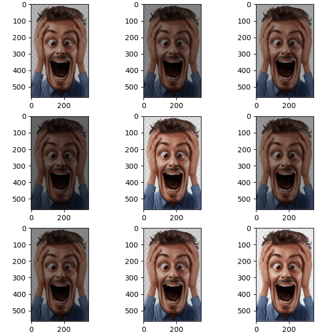
As you can see each of the images above has a different level of brightness.
Cropping the Images Using TensorFlow
Cropping is removing unnecessary borders from the image. Here we will import the MNIST dataset and apply cropping to the images. So, let us first import the dataset.
# importing the module
from tensorflow.keras.datasets import mnist
# Importing the dataset
(x_train, y_train), (x_test, y_test) = mnist.load_data()
# fixing the size of the images
input_image = x_train[0].reshape(28, 28, 1)
As you can see, we have reshaped the very first image from the dataset.
Now, let us build the neural layers and apply the cropping.
# importing the required modules
from tensorflow.keras.models import Sequential
from tensorflow.keras.layers import Cropping2D
# Create the model
model = Sequential()
# cropping the imge in the CNN layer
model.add(Cropping2D(cropping=((7, 7), (7, 7)), input_shape=(28, 28, 1)))
# printing the summay
model.summary()
Output:
Model: "sequential"
_________________________________________________________________
 Layer (type)                Output Shape              Param #
=================================================================
 cropping2d (Cropping2D)     (None, 14, 14, 1)         0

=================================================================
Total params: 0
Trainable params: 0
Non-trainable params: 0
As you can see the size of the image decrease and how its size is 14 by 14.
Now, let us visualize the actual effect of the cropping.
# visualizing the cropped image
model_inputs = np.array([input_image])
# making predictions
outputs_cropped = model.predict(model_inputs)
# getting the first cropped image
outputs_cropped = outputs_cropped[0]
# visualizing both images
fig, axes = plt.subplots(1, 2)
axes[0].imshow(input_image[:, :, 0])
# setting the title
axes[0].set_title('Original image')
axes[1].imshow(outputs_cropped[:, :, 0])
# setting the titile
axes[1].set_title('Cropped input')
fig.suptitle(f'Original and cropped input')
fig.set_size_inches(9, 5, forward=True)
plt.show()
Output:
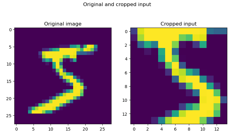
As you can see, the image has been cropped. You may be interested to learn how PCA can be applied to images.
Summary
Image processing using TensorFlow is a technique for applying various procedures to an image in order to improve it or extract some relevant information from it. It is a kind of signal processing where the input is an image and the output can either be another image or features or characteristics related to that image. In this article, we discussed image processing in CNN using TensorFlow. We learn how we can flip, adjust brightness and rotate the image.