Do you want to know what is linear regression, how to implement it in Python, and learn about Hyperparameter tuning of Linear regression? Well, here we go!
A linear regression algorithm in machine learning is a simple regression algorithm that deals with continuous output values. It is a method for predicting a goal value utilizing different variables. The main applications of linear regression include predicting and finding correlations between variables’ causes and effects. In this article, we will do hyperparameter tuning of linear regression algorithms using various simple ways. Before going to the hyperparameter tuning of the linear regression algorithm, we will explain what is linear regression algorithm, how it works, and how we can apply it to various datasets.
What is a Linear Regression Algorithm in Machine Learning?
Linear regression is a supervised machine learning algorithm that is used to make predictions for regression values. A regression operation uses independent variables to model a target prediction value. It is mostly used to determine how variables and output values relate to one another.
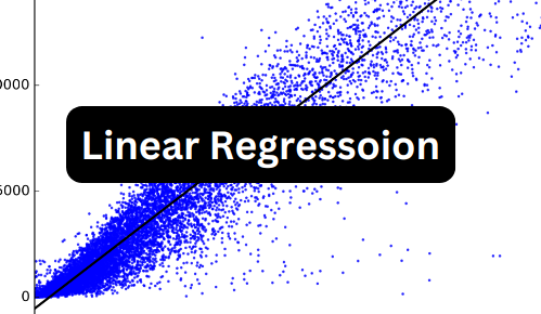
The main task of the linear regression algorithm is to find the best-fitted line for the regression values. For simplicity, you can imagine linear regression as taking x and y values and finding the slope. For example, see the below graph which shows the best-fitted line for the values in the 2D graph.
As you can see, we had various continuous values and then the linear regression finds the best-fitted line for the given values.
Basically, there are two types of linear regression algorithms in machine learning.
- Simple linear regression: In simple linear regression there is only one dependent value for the corresponding dependent value. In other words, there is only one possible value for one x value. A simple linear equation has an x variable and a slope. eg
y = cx + m - Multilinear regression: In multilinear regression, there is more than one independent variable and only one dependent variable. In other words, more than one variable contributes to the output of the y value. A simple multilinear regression can be
y = cx + bz + m
Positive Linear Regression in Machine Learning
When the independent variable rises on the X-axis and the dependent variable also increases on the Y-axis, there is a positive linear relationship. In other words, when the input variables rise, so do the output variables.
Negative Linear Regression in Machine Learning
When the independent variable rises on the X-axis and the dependent variable decreases on the Y-axis, there is a negative linear relationship. In other words, when the input variables rise, at the same time the output variable decreases. Such a linear relationship will have a negative slope.
What is The Equation of Linear Regression in Machine Learning?
As we discussed in the above section that linear regression is simply a slop of the data points. Similarly, the equation of linear regression is the same as for any other slope. But our main focus is not to find the slope in this section, we will use the same equation to find the best-fitted line for our dataset.
y = mx + c
In the above equations:
- Y represents the continuous output value
- c represents the constant value.
- x represents the x value
- m shows the slope of the equation.
So, the linear regression model takes the data with x or input values and y or output values and calculates the m/slope and the constant. It will then uses these values for making predictions about the output when the input value is given.
Linear Regression Algorithm in Machine Learning Using Python
As we discussed linear regression in detail, it is time to jump into the coding part. We will now use Python to implement the linear regression algorithm on various datasets. Before going to the implementation part, ensure you have installed the following required modules on your system.
pip install sklearn
pip install pandas
pip install matplotlib
pip install seaborn
pip install numpy
Once you install the modules, it is time to use them and train our model.
Simple Linear Regression Using Sklearn
For simplicity, we will start implementing simple linear regression. For this purpose, we will use the Bitcoin dataset and we will choose only two columns. You can download the dataset from this link:
Let us import the dataset and print out a few rows to get familiar with the type of dataset.
# importing pandas
import pandas as pd

# loading the dataset
data = pd.read_csv("BTC-USD.csv")

# printing the dataset
data.head()
The dataset contains more than two variables. But for the simple regression, we just need two columns. In this case, we will use the opening price as the input variable and the closing price as the output variable and we will remove all other columns.
# dropping the column values
data.drop('Date', axis=1, inplace=True)
data.drop('Volume', axis=1, inplace=True)
data.drop('High', axis=1, inplace=True)
data.drop('Low', axis=1, inplace=True)
data.drop('Adj Close', axis=1, inplace=True)
As you can see, we have dropped other columns. Let us now visualize the input and output values using a scattered plot.
# importing the module
import matplotlib.pyplot as plt

# fixing the size of plot
plt.Figure(figsize=(10, 8))

# plotting simple scattered plot
plt.scatter(data['Open'], data['Close'])
plt.show()
Output:

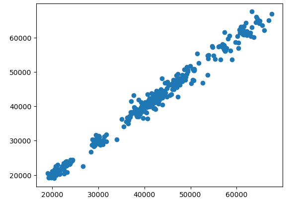
The graph shows that both values are correlated. If your data has some non-numeric values, then you need to convert the non-numeric to numeric values before training the model.
Training Simple Linear Regression Using Sklearn
Before training the simple linear regression, we have to split the dataset into testing and training parts. First, let us divide the data into input and output values.
# input values
X = data.drop('Close', axis=1)

# output values
Y = data.drop('Open', axis=1)
Now, we will split the data into training and testing parts using sklearn module. We will assign value 1 to the random state.
# Splitting the dataset into the Training data set and Testing data set
from sklearn.model_selection import train_test_split

# 30% data for testing, random state 1
X_train, X_test, y_train, y_test = train_test_split(X, Y, train_size=.7, random_state=1)
In the above code, we have split the dataset into testing and training parts and we assigned 30% of the data for the testing.
Now, we will import the linear regression model and will train on the training dataset.
# Importing linear regression form sklear
from sklearn.linear_model import LinearRegression

# initializing the algorithm
regressor = LinearRegression()

# Fitting Simple Linear Regression to the Training set
regressor.fit(X_train, y_train)

# Predicting the Test set results
y_pred = regressor.predict(X_test)
As you can see, the training is complete as we used the testing data to make predictions.
Evaluating Simple Linear Regression
Once the model has predicted the output values, we need to know how well the model has predicted. Let us first visualize the predicted line for the testing data.
You may like the hyperparameter tuning of the KNN algorithm as well.
# plotting the actual values in dotted form
plt.scatter(X_test, y_test, color='red')

# blue line for the best fitted line
plt.plot(X_test, y_pred, color='blue')

# defining the title
plt.title('Open vs Closing price')

# showing the graph
plt.show()
Output:

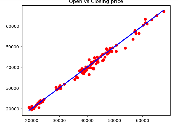
The blue line shows the predicted line for the red dots which are the testing points. Let us also visualize the actual and predicted values using a line plot to see how close they are close to each other.
# import numpy
import numpy as np

# figure size
plt.figure(figsize=(12, 8))

# acutal values
plt.plot([i for i in range(len(y_test))],np.array(y_test), c='g', label="actual values")

# predicted values
plt.plot([i for i in range(len(y_test))],y_pred, c='m',label="predicted values")
plt.legend()
plt.show()
Output:

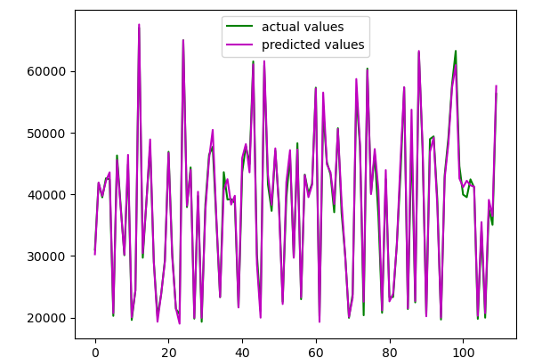
As you can see, the predicted values are very much close to the actual values. Let us use some evaluation matrix to evaluate our model.
# Importing mean_absolute_error from sklearn module
from sklearn.metrics import mean_squared_error, mean_absolute_error

# printing the mean absolute error
print(mean_absolute_error(y_test, y_pred))
print(mean_squared_error(y_test, y_pred))
Output:
894.538275
1601183.85745374
Multilinear Regression Using Sklearn
Now we will dataset with multiple columns/input values to predict one output. The process is very much similar to the training of the simple regression one except that this time we will take a dataset with multiple columns.
Let us again, load the dataset and print a few rows.
# loading the dataset
data = pd.read_csv("BTC-USD.csv")

# dropping columns
data.drop('Date', axis=1, inplace=True)

# printing the dataset
data.head()
This time, we will not drop any column and will use all the input columns to train the linear regression model.
Training the Multilinear Regression Model in Sklearn
Let us first split the dataset into testing and training parts as we did for the simple linear regression model.
# dividing the dataset
X = data.drop('Close', axis=1)
Y = data['Close']

# 30% data for testing, random state 1
X_train, X_test, y_train, y_test = train_test_split(X, Y, train_size=.7, random_state=1)
Once the splitting is complete, the next step is to use the training dataset to train the linear regression model.
# initializing the algorithm
regressor = LinearRegression()

# Fitting Simple Linear Regression to the Training set
regressor.fit(X_train, y_train)

# Predicting the Test set results
y_pred = regressor.predict(X_test)
Once, the training and predicting are complete we can then use various evaluation matrices to evaluate the performance of the model.
Evaluating the Multilinear Regression Model
Let us first visualize the actual and predicted values using matplotlib.
# import numpy
import numpy as np

# acutal values
plt.plot([i for i in range(len(y_test))],np.array(y_test), c='g', label="actual values")

# predicted values
plt.plot([i for i in range(len(y_test))],y_pred, c='m',label="predicted values")
plt.legend()
plt.show()
Output:

As you can see, this time our model was very accurate and predicted the closing price very accurately.
Let us also use different evaluation matrices to find the performance of the model.
# Importing mean_absolute_error from sklearn module
from sklearn.metrics import mean_squared_error, mean_absolute_error

# printing the mean absolute error
print(mean_absolute_error(y_test, y_pred))
print(mean_squared_error(y_test, y_pred))
Output:
3.954358473
3.45335455
As you can see, we get really small values for the mean absolute error and mean squared error because our model was very much accurate in predicting the closing price.
How to do Hyperparameter Tuning of Linear Regression?
Hyperparameter is applied in linear regression in order to maximize the performance of the model without overfitting and reduce the variance error. Variance refers to the amount that the predicted value would change if different training data were used. while Bias refers to the amount that the predicted value would change if different training data were used.
The question is how to maximize the performance of the model without overfitting it. The answer is using Regularization techniques.
Regularization lessens the model’s tendency toward overfitting. This is done even if the model is accurate in order to stop the issue from happening again. This is done by adding more errors and forcing the model to learn more. The model will get more knowledge as a result. As a result, the model will be able to analyze additional data without any problems if it is added at a later time. The model’s performance will now improve and surpass that of the unregularized model.
How does the regularization work?
Every time we regularize, the coefficient decreases. By over-tuning in alpha, we must also be careful to avoid under-fitting our model. A punishment factor is an alpha. By creating a line that doesn’t contact the majority of the points, the error is introduced into the system. As these regularization models construct models that lessen the slope, which will not vary significantly for fresh data, they will decrease the coefficient. The variables completely determine how much a coeff shrinks.
If a feature is important, shrinkage will be less, however, if a feature is not important, shrinkage would be more. When a feature is extremely insignificant, the coefficient will equal zero. This regularizes models, which has the benefit that the model will complete all the work even if the assumptions are not tested.
There are basically two types of regularization:
- Ridge Regularization: It adds the “Squared magnitude” of the coefficient as a penalty term to the loss function. It is called an L2 penalty
- Lasso regularization: The (least absolute shrinkage and selection operator) adds the “Absolute value of magnitude” of the coefficient as a penalty term to the loss function. It is called an L1 penalty.
Now the question is how to find the best alpha values. Well, in machine learning, gradient descent is an iterative optimization process that reduces a loss function. Gradient descent is used to discover the optimal set of parameters, and the loss function quantifies how well the model will perform given the present set of parameters (weights and biases).
Summary
Linear regression is a simple Machine learning algorithm that is used for continuous or regression problems. In this article, we discussed how we can use linear regression, and train the model on a simple and multilinear dataset. Also, we discussed how we can evaluate the performance of the model using various evaluation matrices. Toward the end, we also discussed how we can do hyperparameter tuning of linear regression in machine learning.

