Investors purchase and sell company shares on the stock market. Companies provide shares and other securities for trading on a series of exchanges. Additionally, it incorporates over-the-counter (OTC) markets where investors conduct direct securities transactions with one another (rather than through an exchange). So, It is always important to know how to analyze the stock market so that the company will get more benefits.
In this article, we will learn how we can analyze the stock market using Machine learning concepts. More specifically, we will be using the two most important algorithms to analyze stock market which are ARIMA and Facebook Prophet. We will learn how we can use these two algorithms to analyze stock market, visualize the dataset and interpret various plots.
Top 6 Machine learning algorithms to analyze stock market in Python
Primary Skills Needed to Analyze Stock Market Price Using Machine Learning
Because our focus is to analyze stock market using Python and Machine learning algorithms, so we already assume that you have a basic understanding of Python programming language and Machine learning. Although you don’t need to be super smart and good at Machine learning and Python in order to analyze stock market. So, before moving to the main part of the article, make sure that you have a basic understanding of the following topics.
- Python to visualize: You can use any of the modules in Python for visualization but make sure that you have a basic understanding of how visualization in Python works. Check out Pandas for visualization, 3D graphs in Python, and Python plots on a google Map.
- Basic knowledge of Machine Learning: We assume that you have a basic understanding of Machine learning models, especially supervised learning models.
- Analytical skills: The final and most important skill to analyze stock market is analytical skills. You should be able to analyze and interpret the various graphs.

Machine Learning Algorithms to Analyze Stock Market
The practice of foreseeing the future value of a stock traded on a stock exchange in order to make money is known as stock price prediction using machine learning. It is difficult to predict stock values with great accuracy because of the many elements that are involved. But thanks to Machine Learning algorithms that help us to analyze stock market. There are various algorithms in Machine learning that can be very useful in making predictions and analyzing the stock market but in this article, we will be discussing the following two machine learning algorithms to analyze stock market.
- ARIMA
- Facebook Prophet
ARIMA Algorithm to Analyze Stock Market
ARIMA stands for Autoregressive Integrated Moving Average. It is a statistical analysis model that helps us to understand the time series data in-depth and helps us to predict the future forecast as well. It takes past values, analyzes them, and predicts the future.
The ARIMA models are comprised of three important terms. And these terms are usually represented as p, d, and q terms where:
- p represents the AR ( auto-regressive) term.
- d represents the number of differencing required to make the time series stationary.
- q represents the order of the MA ( moving average) term.
One of the important things to note is that ARIMA models can only be applied to stationary time series. A stationary time series is simply a time series that does not depends on the context or the time at which the data was taken. In other words, we can say that the data shouldn’t depend on seasons or months.
Importing and Analyzing the Time Series Dataset
We will use the Bitcoin dataset from Sep 2021 to Sep 2022. You can download the dataset from here. Let us first import the dataset and print out a few rows to get familiar with the time series dataset.
# importing pandas module
import pandas as pd

# importing the time series dataset
data = pd.read_csv("BTC-USD.csv")

# printing
data.head()
Output:

As you can see, we have a number of columns representing different prices. All we need for this article is the first column and the closing price of the Bitcoin. So, let us drop other columns.
# dropping columns
data.drop('Open', inplace=True, axis=1)
data.drop('High', inplace=True, axis=1)
data.drop('Low', inplace=True, axis=1)
data.drop('Adj Close', inplace=True, axis=1)
data.drop('Volume', inplace=True, axis=1)

# printing few rows
data.head()
Output:

As you can see, we have now only the date and closing price for Bitcoin. Let us now move forward and start analyzing Bitcoin’s price using the ARIMA model.
As we said, the ARIMA model consists of three important terms. In the upcoming sections, we will explore each of these terms.
How to find Oder of Differencing in the ARIMA Model?
As we discussed in the beginning that the ARIMA model takes three parameters which are p, d, and q. Where the d represents the order of differencing in the ARIMA model to make the time series a stationary time series.
While finding the order of differencing in the ARIMA model, we should find the minimum number of differencing that will make data a stationary time series. But before moving to find the order of differencing, we need to check if the data is already stationary. If the data is already stationary then no need to find the order of differencing and in such case, the value of d will be zero.
We will use Augmented Dickey-Fuller Test to check if the time series is stationary or not. It is one of the most commonly used statistical tests when it comes to analyzing the stationary of a series. The null hypothesis of the ADF test is that the time series is non-stationary. The null hypothesis is rejected and it is concluded that the time series is stationary if the test’s p-value is less than the significance level (0.05).
# importing the required modules
from statsmodels.tsa.stattools import adfuller
from numpy import log

# dropping the null values
result = adfuller(data.Close.dropna())

# finding the p-value
print('ADF Statistic: %f' % result[0])
print('p-value: %f' % result[1])
Output:

As you can see, the p-value is more than 0.05 which means our data is not stationary. Now, let us differentiate the time series and see what the autocorrelation plot looks like.
We will differentiate two times the series and plot the graph for each of the differentiations.
# Importing the modules
from statsmodels.graphics.tsaplots import plot_acf, plot_pacf
import matplotlib.pyplot as plt

# Size of the time series plots
plt.rcParams.update({'figure.figsize':(7,6), 'figure.dpi':120})


# plotting original time series data
fig, axes = plt.subplots(3, 2, sharex=True)

# labeling the original data
axes[0, 0].plot(data.Close); axes[0, 0].set_title('Original Series')
plot_acf(data.Close, ax=axes[0, 1])

# first differenciating to make the data stationary
axes[1, 0].plot(data.Close.diff()); axes[1, 0].set_title('1st Order Differencing')
plot_acf(data.Close.diff().dropna(), ax=axes[1, 1])


# 2nd Differencing
axes[2, 0].plot(data.Close.diff().diff()); axes[2, 0].set_title('2nd Order Differencing')
plot_acf(data.Close.diff().diff().dropna(), ax=axes[2, 1])
plt.show()
plt.show()
Output:

As you can see, after the second differentiation the time series become stationary. So, this means we will take the d value as 2.
How to Find the Order of the AR Term in the ARIMA Model?
In the next step, we will find out if we need an AR term or not. If we need the AR term then what should be the order of the AR term? We will use the partial autocorrelation plot to find the order of the AR term. A partial autocorrelation is a summary of the relationship between an observation in a time series with observations at prior time steps with the relationships of intervening observations removed.
In other words, partial autocorrelation is the relation between observed at two-time spots given that we consider both observations to be correlated to the observations at other time spots. The significant threshold value is displayed in the light blue area of the partial autocorrelation plot, and each vertical line represents the PACF values at each time location. The only vertical lines in the plot that are noteworthy are those that go beyond the area in light blue.
Let us now plot the partial correlation plot to find the AR term. To make things simpler, we will take the first differentiation as stationary data.
#importing the module
from statsmodels.graphics.tsaplots import plot_acf, plot_pacf

# partial correlation of first term
plt.rcParams.update({'figure.figsize':(7,3), 'figure.dpi':120})
fig, axes = plt.subplots(1, 2, sharex=True)

# plotting on differen axis
axes[0].plot(data.Close.diff()); axes[0].set_title('1st Differencing')
axes[1].set(ylim=(0,5))

# plotting partial autocorrelation function
plot_pacf(data.Close.diff().dropna(), ax=axes[1])
plt.show()
Output:

The significant threshold value is displayed in the light blue area of the partial autocorrelation plot, and each vertical line represents the PACF values at each time location. The only vertical lines in the plot that are noteworthy are those that go beyond the area in light blue. We can see that the very first line is far away from the light blue area, so we can take the order of the AR term as 1.
How to Find the Order of MA Term in the ARIMA Model?
The third most important term in the ARIMA model is the MA (moving average). We already had found the p and d order. Now, we will find the order of the MA term. We use ACF (autocorrelation function) plots to find the order of the MA term. The autocorrelation function (ACF) defines how data points in a time series are related, on average, to the preceding data points.
# setting the size
plt.rcParams.update({'figure.figsize':(9,3), 'figure.dpi':120})

#  fixing the subplots
fig, axes = plt.subplots(1, 2, sharex=True)
axes[0].plot(data.Close.diff()); axes[0].set_title('1st Differencing')
axes[1].set(ylim=(0,1.2))

# plotting the autocorrelation function
plot_acf(data.Close.diff().dropna(), ax=axes[1])
plt.show()
Output:

As you can see, the first line is quite away from the light blue area, so we can fix the value of q as 1.
Creating ARIMA Model
As we have found the values for all the necessary parameters of ARIMA ( p=1, d = 1, q =1), we can move forward and build the ARIMA model to forecast the values.
# importing the module
import statsmodels.api as sm
from statsmodels.graphics.tsaplots import plot_predict

# values of p, d, and q
ARIMA_model = sm.tsa.arima.ARIMA(data.Close, order=(1,1,1))

# Training process
model_fit = ARIMA_model.fit()

# arima model results
plot_predict(model_fit,dynamic=False)
plt.show()
Output:

As you can see, our model has predicted the values with a 95% confidence interval.
Facebook Prophet to Analyze Stock Market
Facebook Prophet is an open-source time-series modeling method that combines some traditional concepts with some modern innovations. It does not suffer from some of the aforementioned shortcomings of other algorithms and excels at modeling time series with numerous seasonalities. Some of the main features of the Facebook prophet are:
- It is accurate and much faster than other forecasting algorithms
- It allows customizing the parameters
- It helps to deal with seasonalities in the time series data
- The holiday function allows Prophet to adjust forecasting when a holiday or major event may change the forecast
- One of the important features of the Facebook prophet is that it can handle outliers by itself.
- It also has a feature to detect the change points automatically.
Now, let’s jump into the analyzing part and analyze the dataset about Bitcoin in depth using the Facebook Prophet.
How to Train the Facebook Prophet on a Time Series Dataset?
Let us now explore how we can train the model using a time series dataset. Before training the model, make sure that the names of the columns are ds ( for date) and y ( for output values). Because by default, the Facebook prophet can only take the data with ds and y column names. So, first, let us change the column names.
# changing the column name
data.rename(columns={'Date':'ds','Close':'y'},inplace=True)
Now, let us train the model on the dataset. We will use 95% of the confidence level in the training process.
# importing the module
from prophet import Prophet

# 95% confidence interval
model = Prophet(interval_width= 0.95)

# training the model
model.fit(data)
Once the training is complete, we can then use our model to predict the forecast and visualize the data in more depth to understand the trend in more detail.
# forecasting for future
future = model.make_future_dataframe(periods=3, freq='M')

# forecast predictions
forecast = model.predict(future)

# prediction head
forecast.head()
Output:

As you can see, there are many more data have been added to the forecast rather than just the two columns. It shows the overall trend, upper limit, lower limit, yearly trend, weekly trend, and many more. In this article, we will analyze a few of them but you can go through all of them and analyze them separately to get an in-depth understanding of the time series data.
Visualizing the Time Series Using Facebook Prophet
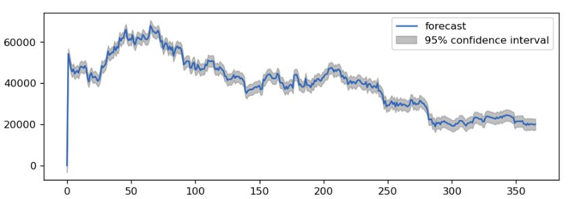
Let us first visualize the forecasting of the Facebook prophet mode.
# visualizing the forecat predictions
forecasting = model.plot(forecast)
Output:

As you can see, the prophet was able to predict future values with a 95% confidence interval.
Another cool feature of the Facebook prophet that helps us to analyze the stock market is its ability to divide the data into components. Let us now visualize the dataset in different components.
# yearly and weekly seasonality
components = model.plot_components(forecast)
Output:

The first plot shows how the price of Bitcoin changes over the year ( months) while the second graph is more interesting. It shows how the price changes over weeks. It shows that mostly the price of Bitcoin is at its peak on Wednesday while it declined to its lowest point on Friday. That means buying Bitcoins on Friday and selling them on Wednesday will always give benefits.
The next important feature of the Facebook prophet that can help us to analyze the data is its ability to detect the change points. The change points are some abrupt changes in the time series dataset.
# import the ploting module
from prophet.plot import add_changepoints_to_plot

# creating plot
change_points = model.plot(forecast)

# completely automatic forecasting techniques
change_points = add_changepoints_to_plot(change_points.gca(), model, forecast)
Output:

As you can see, the model was able to detect the change points in our time series dataset.
NOTE: You can access all the source code from my GitHub account. Please don’t forget to follow and give me a star.
Summary
The stock market enables businesses to raise funds by selling stock shares and corporate bonds, and it gives investors a chance to profit from the business’s financial success through capital gains and dividend payments. So, it is important to learn how to analyze the stock price. In this short article, we discussed two different machine-learning approaches to analyzing the stock market.
2 thoughts on “ARIMA and Facebook Prophet in Machine Learning”