LightGBM is a supervised boosting algorithm, that was developed by the Mircosoft company and was made publically available in 2017. It is an open-source module that can be used as a boosting model. It is very powerful, fast, and accurate as compared to many other boosting algorithms. In this article, we will go through some of the features of the LightGBM that make it fast and powerful, and more importantly we will use various methods for hyperparameter tuning of LightGBM including custom and GridSearchCV methods. We will also implement LightGBM on regression and classification datasets and evaluate the models.
Before going into LightGBM, make sure that you have gone through all the boosting algorithms that we covered in the previous articles. The lightGBM is mostly more powerful than XGBoost, Gradient boost, and Ada boost on many testing data samples. Also, make sure you have a strong knowledge of decision trees and random forest algorithms, as LightGBM uses random trees as weak learners.
What is LightGBM?
The LightGBM is short for Light Gradient Boosting Machine. It is a supervised boosting algorithm that works in a similar way as the XGBoost algorithm does but with some advanced features that make it more powerful and fast.
Similar to the XGBoost algorithm, we don’t need to handle the NULL value explicitly in the data preprocessing step while using the LightGBM algorithm as it also handles NULL values automatically.
Other important features that make LightGBM different from other boosting algorithms is that it uses a histogram-based algorithm for the splitting of nodes and Gradient-Based One Side Sampling (GOSS) for the sampling.
How to Implement LightGBM in Python?
The implementation of LightGBM in Python is very easy. All we need to do is first install the LightGBM module on our system using the pip command. We will follow the following steps to implement the LightGBM on regression and classification datasets.
- Import and explore the dataset
- Split the dataset into testing and training parts
- Training the model on the training dataset
- Testing and evaluating the model using the testing dataset
- Hyperparameter of the model to get an optimum result.
LightGBM Classifier Using Python
Now, we will use the LightGBM classifier to classify the dataset. For the understanding purpose, we will use the iris dataset. The dataset contains information about three different types of flowers. Before going to the implementation part, make sure that you have installed the following Python modules on your system as we will be using them for implementation purposes.
- lightgbm
- sklearn
- matplotlib
- pandas
- numpy
- seaborn
You can use the pip command to install the required modules.
Let us first load the dataset and then explore it.
# importing the required modules
from sklearn import datasets
import pandas as pd
import numpy as np

# loading the iris dataset
dataset = datasets.load_iris()

# converting the data to DataFrame
data = pd.DataFrame(data= np.c_[dataset['data'], dataset['target']],
                     columns= dataset['feature_names'] + ['target'])

# printing the few rows
data.head()
Four input variables contain information about the length and width of sepals and petals of three different kinds of flowers. You can use pandas for visualization or matplotlib module to visualize the dataset for more insights.
Now, we will split the dataset to use it for testing and training purposes. But before it, we must divide the dataset into input and output variables.
# splitting the dataset into input and output
Input = data.drop('target', axis=1)
Output =data['target']
Once, we have divided the input and output variables, it is time to split the dataset into the testing and training parts so that we can use the training part to train the model and then use the testing dataset to test the model. We will also assign value 1 to the random state.
# importing the module
from sklearn.model_selection import train_test_split

# splitting into testing and training parts
X_train, X_test, y_train, y_test = train_test_split(Input, Output, test_size=0.30, random_state=1)
As you can see, we have assigned 30% of the dataset to the testing part and 70% of the dataset to the training part.
Training the LightGBM Classifier
Let us now import the LightGBM classifier and train the model on the training dataset.
# importing the lightgbm module
import lightgbm as lgb

# initializing the model
model_Clf = lgb.LGBMClassifier()

# training the model
model_Clf.fit(X_train, y_train)
This will take some time and once the training is complete, we can then use the testing dataset to evaluate the performance of the model.
Evaluating the Performance of the LightGBM Classifier
Let us make predictions for the output values using the testing dataset.
# making prediction
clf_pred = model_Clf.predict(X_test)
To know how well these predictions are, we will use different evaluation matrices. First, let us visualize the predictions and the actual values using a confusion matrix. The simplest way to understand the confusion matrix is that any value in the main diagonal is the correctly classified value and all values/predictions other than the main diagonal one are incorrectly classified ones.
# importing modules
import matplotlib.pyplot as plt
from sklearn.metrics import confusion_matrix, ConfusionMatrixDisplay

# confusion matrix plotting
cm = confusion_matrix(y_test, clf_pred, labels=model_Clf.classes_)

# labelling
disp = ConfusionMatrixDisplay(confusion_matrix=cm, display_labels=model_Clf.classes_)
disp.plot()
plt.show()
Output:
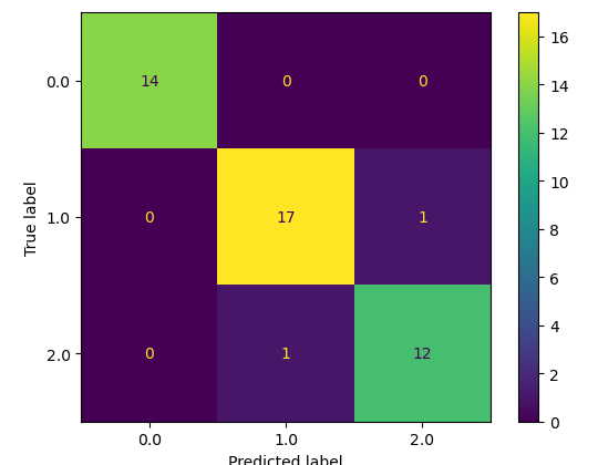
As you can see, only one prediction was incorrect and all others were correctly classified. Let us also find the accuracy score of the model.
# importing the module
from sklearn.metrics import accuracy_score

# printing
print("The accuracy is: ", accuracy_score(y_test, clf_pred))
Output:
The accuracy is : 0.97777777
As you can see, we have an accuracy score of 97% which means 97% of the testing dataset was correctly classified by the model.
LightGBM Regressor Using Python
Now, we will use the LightGBM regressor and implement it on a regression dataset. The dataset contains information about the price of houses in Dushanbe city. Let us first import the dataset.
# importing dataset
data = pd.read_csv('house.csv')

# heading of the dataset
data.head()
As you can see multiple factors contribute to the price of the house. Also, notice that there are some null values as well and we don’t need to handle them here as the LightGBM handles the null values automatically.
Splitting the Dataset
Similar to what we did before, we will divide the dataset into input and output values and then split the data set into the testing and training parts
# input and output variables
Input = data.drop('price', axis=1)
Output = data.price
Now we will split the dataset into testing and training parts.
# importing the module
from sklearn.model_selection import train_test_split

# splitting into testing and training parts
X_train, X_test, y_train, y_test = train_test_split(Input, Output, test_size=0.25)
Now let us go to the training part of the lightGBM regressor.
Training the LightGBM Regressor
First, we have to initialize the LightGBM regressor and then train the model on the training dataset.
# initialzing the model
model_reg = lgb.LGBMRegressor()

# train the model
model_reg.fit(X_train,y_train)
Once the model is trained, we can then use the testing dataset to make predictions.
# Making predictions
reg_pred = model_reg.predict(X_test)
Now, we will use various evaluation matrices to evaluate the performance of the model.
Evaluating the LightGBM Regressor
The best way to see the performance of the model is to visualize the actual and the predicted values. We will use the matplotlib module to visualize the actual and the predicted values.
# importing the module
import matplotlib.pyplot as plt

# acutal values
plt.plot([i for i in range(len(y_test))],y_test, c='g', label="actual values")

# predicted values
plt.plot([i for i in range(len(y_test))],reg_pred, c='m',label="predicted values")
plt.legend()
plt.show()
Output:
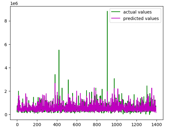
The actual and predicted values are pretty much close. Let us also find the R-square of the model.
#importing the r-square score
from sklearn.metrics import r2_score

# calculating the r score
print('R score is :', r2_score(y_test, reg_pred))
Output:
R Score is : 0.627
As you can see we get a high value of R-square which means the model has predicted very well.
Comparing lightGBM With Other Boosting Algorithms
Let us now compare the lightGBM with other boosting algorithms that we studied in the previous articles. We will use the LightGBM regressor which we had trained in the above section and compare its results with other boosting algorithms. Mainly we will be comparing the LightGBM with the following boosting algorithms.
- LightGBM vs AdaBoost
- LightGBM vs Gradient Boost
- LightGBM vs XGBoost
LightGBM vs XGBoost Algorithm
We assume that you already have enough knowledge of the XGBoost algorithm. You can read about the working, implementation, and hyperparameter tuning of XGBoost from the article XGBoost using Python.
Let us import the XGBoost and train on the training dataset.
# importing the module
import xgboost as xgb

# xgboost regressor
model = xgb.XGBRegressor()

# training the model
model.fit(X_train,y_train)

# making predictions
xgboost_pred = model.predict(X_test)
Let us now visualize the XGBoost and LightGBM predictions to see which one is close to the actual values.
# importing the module
import matplotlib.pyplot as plt

# figure size
plt.figure(figsize=(12, 8))

# acutal values
plt.plot([i for i in range(len(y_test))],y_test, label="actual values")

# predicted values
plt.plot([i for i in range(len(y_test))],reg_pred, c='m',label="predicted values")

# predicted values
plt.plot([i for i in range(len(y_test))],xgboost_pred, c='g',label="predicted values")
plt.legend()
plt.show()
Both models predicted the output values really well. We will also calculate the R-square score.
# calculating the r score
print('R score of lightGBM :', r2_score(y_test, reg_pred))
print('R score of XGBoost :', r2_score(y_test, xgboost_pred))
Output:
R score of lightGBM : 0.627
R score of XGBoost : 0.612
As you can see, the R-square score of lightGBM is slightly higher than the XGBoost which means the predictions of the lightGBM are closer to the actual values than the predictions of the XGBoost.
LightGBM vs Gradient Boosting algorithm
Now, we will compare the LightGBM model with the Gradient boosting algorithm. We assume that you already have been through the article about gradient boosting algorithms and have a solid understanding of their work. You can check the working, implementation, and hyperparameter tuning of the Gradient boosting algorithm from the article Gradient boosting algorithm using Python.
We have to do one data preprocessing step before training the Gradient boosting algorithm. As we had null values in our dataset, the Gradient boosting algorithm cannot handle null values so, we have to remove them from the dataset before training the model.
Let us import the Gradient boosting algorithm and train the model using the training dataset.
# importing the regressor
from sklearn.ensemble import GradientBoostingRegressor

# training the model with 2 iterations
GB_rgsr=GradientBoostingRegressor()

# training the model
GB_rgsr.fit(X_train,y_train)

# making the predictions
GB_predict=GB_rgsr.predict(X_test)
Let us again visualize the predictions of the LightGBM and Gradient boosting algorithm.
# figure size
plt.figure(figsize=(12, 8))

# acutal values
plt.plot([i for i in range(len(y_test))],y_test, label="actual values")

# predicted values
plt.plot([i for i in range(len(y_test))],reg_pred, c='m',label="LightGBM")

# predicted values
plt.plot([i for i in range(len(y_test))],GB_predict, c='g',label="Gradient boost")
plt.legend()
plt.show()
The predictions of the lightGBM are closer to the actual values than the Gradient-boosting one. Let us also calculate the R-square score for both of the models.
# calculating the r score
print('R score of lightGBM :', r2_score(y_test, reg_pred))
print('R score of Gradient boost :', r2_score(y_test, GB_predict))
Output:
R score of lightGBM : 0.627
R score of Gradient boost : 0.515
As you can see, the R-square score of lightGBM is higher than the gradient boosting model.
LightGBM vs. AdaBoost Algorithm
Let us now compare the AdaBoost model with LightGBM one. We assume that you have already been through the AdaBoost algorithm and have solid knowledge. You can read about the working, implementation, and hyperparameter tuning of the AdaBoost from the article AdaBoot using Python.
# importing ada boost regressor
from sklearn.ensemble import AdaBoostRegressor

# Create adaboot
Ada_regressor = AdaBoostRegressor()

# training the ada boost regressor
AdaBoost = Ada_regressor.fit(X_train, y_train)

#Predict price
AdaBoost_pred = AdaBoost.predict(X_test)
Let us also calculate the R-square score of both models.
# calculating the r score
print('R score of lightGBM :', r2_score(y_test, reg_pred))
print('R score of Ada boost :', r2_score(y_test, AdaBoost_pred))
Output:
R score of LightGBM : 0.627
R score of Ada boost: 0.093
R-square shows that the LightGBM has performed much better than the AdaBoost.
Hyperparameter Tuning of LightGBM
Hyperparameter tuning is finding the optimum values for the parameters of the model that can affect the predictions or overall results. In this section, we will go through the hyperparameter tuning of the LightGBM regressor model. We will use the same dataset about house prices. Learn how to tune the classifier model from hyperparameter tuning of boosting algorithms.
Before going to the hyperparameter tuning of LightGBM, let us import all the necessary modules that we will be using in the implementation part.
# importing all the necessary modules  - Hyperparameter Tuning of LightGBM
from numpy import mean
from sklearn.datasets import make_classification
from sklearn.model_selection import cross_val_score
from sklearn.model_selection import RepeatedStratifiedKFold
from matplotlib import pyplot
from sklearn.tree import DecisionTreeClassifier
from sklearn.model_selection import GridSearchCV
from numpy import arange
Let us also create a validation function that will validate the models based on the cross-validation method.
# function for the validation of model - Hyperparameter Tuning of LightGBM
def evaluate_model(model, Input, Ouput):

    # defining the method of validation
    cv = RepeatedStratifiedKFold(n_splits=10, n_repeats=3)


    # validating the model based on the accurasy score
    r_square = cross_val_score(model, Input, Ouput, scoring='r2', cv=cv, n_jobs=-1)

#     returning the accuracy score
    return r_square
Now let us go through some of the important parameters of the LightGBM model to find the optimum values.
Optimum Number of Iterations Using Hyperparameter Tuning of LightGBM
One of the parameters that affect the overall results of the LightGBM is the total number of iterations. So, let us first create a function that will return models with a different number of iterations
# fuction to create models
def build_models():

#     dic of models
    models = dict()

    # number of decision stumps
    decision_stump= [10, 50, 100, 500, 1000]

#    using for loop to iterate though trees
    for i in decision_stump:

#         building model with specified trees
        models[str(i)] = lgb.LGBMRegressor(n_estimators=i)

#     returning the model
    return models
Now, we will call the validation function that we had created before and then the above function to get the optimum number of iterations for the LightGBM model.
# calling the build_models function
models = build_models()

# creating list
results, names = list(), list()

# using for loop to iterate thoug the models
for name, model in models.items():

    # calling the validation function
    R_square = evaluate_model(model, Input, Output)


    # appending the accuray socres in results
    results.append(R_square)
    names.append(name)


    # printing the accuracy score - Hyperparameter Tuning of LightGBM
    print('Iterations (%s)---R-square( %.5f)' % (name, mean(R_square)))
We get optimum results when the number of iterations is 50. Let us also visualize the same information in the box plot as well.
Optimum Number of Features Using Hyperparameter Tuning of LightGBM
Selecting a different number of features also affects the training and predictions of the LightGBM model. So, let us create a function that will return models with a different number of features. In our case, we can only specify the features from 1-5 as our dataset has at most 5 input features.
# creating the function
def build_models():

#     creating dic of models
    models = dict()

    # explore features numbers from 1-5
    for i in range(1,6):

#         appending the models
        models[str(i)] = lgb.LGBMRegressor(max_features=i)

#     returining the models
    return models
Now, let us call the above function and then the validation function.
# calling the function
models = build_models()
# creating the list
results, names = list(), list()
# for loop to iterate through the models
for name, model in models.items():
# calling the evaluting function
R_square = evaluate_model(model, Input, Output)
# storing the accurcy
results.append(R_square)
names.append(name)
# printing - Hyperparameter Tuning of LightGBM
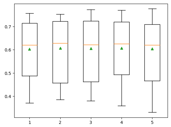
print('---->Features(%s)---R_square( %.5f)' % (name, mean(R_square)))We get optimum results when we use all 5 input values. Now, let us visualize the same information using the box plot as well.
# plotting box plot of the
plt.boxplot(results, labels=names,showmeans=True)

# showing the plot
plt.show()
Output:
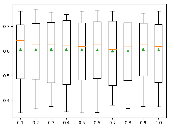
Optimum Sample Size Using Hyperparameter Tuning of LightGBM
Let us now create a function that will return models with different sample sizes.
# creating the function
def build_models():

#     dic of models
    models = dict()

#     exploring different sample values
    for i in arange(0.1, 1.1, 0.1):

#         key value
        k = '%.1f' % i

#     appending the model
        models[k] = lgb.LGBMRegressor(subsample=i)
    return models
Now, we will call the evaluating function and the above function to get the optimum size of the sample.
# calling the function
models = build_models()
# creating the list
results, names = list(), list()
# for loop to iterate through the models
for name, model in models.items():


    # calling the evaluting function
    R_square = evaluate_model(model, Input, Output)

#     storing the accurcy
    results.append(R_square)
    names.append(name)

#     printing - Hyperparameter Tuning of LightGBM
    print('Samples(%s)---R_square( %.5f)' % (name, mean(R_square)))
The R-square is nearly constant for all values of samples. Let us also visualize the same information using a box plot.
# plotting box plot of the
plt.boxplot(results, labels=names,showmeans=True)

# showing the plot
plt.show()
Output:
Optimum Learning Rate Using Hyperparameter Tuning of LightGBM
One of the most important parameters that affect the overall results of the ML model is the learning rate. Let us create a function that will return multiple models with different learning rates.
# creating function
def build_models():

#     creating dic of models
    models = dict()

#     different learning rates
    for i in [0.0001, 0.001, 0.01, 0.1, 1.0]:

#         key value
        k = '%.4f' % i

#     appending the models
        models[k] = lgb.LGBMRegressor(learning_rate=i)
    return models
Now, we will call the above function and the validation function to get the optimum learning rate for the model.
# calling the function
models = build_models()
# creating the list
results, names = list(), list()
# for loop to iterate through the models
for name, model in models.items():


    # calling the evaluting function
    R_square = evaluate_model(model, Input, Output)

#     storing the accurcy
    results.append(R_square)
    names.append(name)

#     printing - Hyperparameter Tuning of LightGBM
    print('Learning Rate(%s)---R Square( %.5f)' % (name, mean(R_square)))
We get an optimum R-square score when the learning rate is 1. Let us also visualize the same information using the box plot.
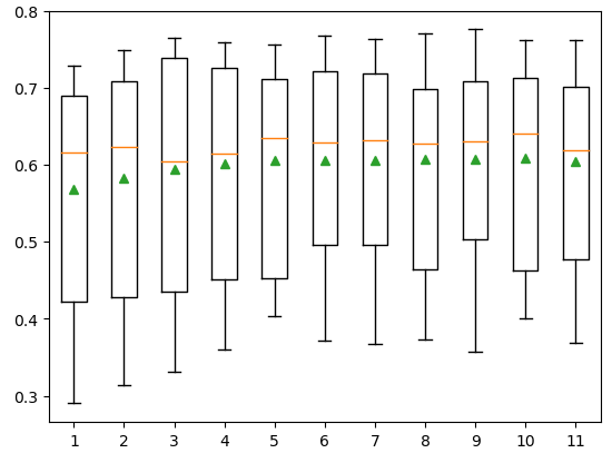
Optimum Depth of the Tree Hyperparameter Tuning of LightGBM
The depth of the decision tree also plays an important role in training the model. Let us create a function that will return multiple models with different depths of decision trees.
# building function for the model
def build_models():

#     creating dic of models
    models = dict()

#     specifying the depth of trees
    for i in range(1,12):

#         appending the models
        models[str(i)] = lgb.LGBMRegressor(max_depth=i)

#   returining the model
    return models
Now, we will call the evaluation function and the above function to get the optimum depth of the decision trees.
# calling the function
models = build_models()

# creating lists
results, names = list(), list()

# iterating through the models
for name, model in models.items():

    # calling the evalution function
    R_square = evaluate_model(model, Input, Output)

    # appending the results
    results.append(R_square)
    names.append(name)

#     printing the results - Hyperparameter Tuning of LightGBM
    print('Decision tree depth (%s)---R_square( %.5f)' % (name, mean(R_square)))
Let us also visualize the same information using the box plot.
# plotting box plot of the
plt.boxplot(results, labels=names,showmeans=True)

# showing the plot
plt.show()
Output:
GridSearchCV in LightGBM to Get Optimum Values for Parameters
GridSearchCV is an algorithm that takes different values for the specified parameters and then returns the optimum combinations. Let us apply the GridSearchCV to find the optimum values for parameters in LightGBM.
Let us first create a LightGBM model and then initialize a range of values for different parameters
# defiing the model
model = lgb.LGBMRegressor()


# creating a dict of grids
grid = dict()

# values for iteration
grid['n_estimators'] = [10, 50, 100, 500]

# values for learning rate
grid['learning_rate'] = [0.0001, 0.001, 0.01, 0.1, 1.0]

# values for the sampel
grid['subsample'] = [0.5, 0.7, 1.0]

# values for teh depth of tree
grid['max_depth'] = [3, 4, 5]
Let us now use the GridSearchCV to find the optimum values for the parameters.
# defining the cv
cv = RepeatedStratifiedKFold(n_splits=10, n_repeats=3)


# applying the gridsearchcv method
grid_search = GridSearchCV(estimator=model, param_grid=grid, n_jobs=-1, cv=cv, scoring='r2')

# storing the values
grid_result = grid_search.fit(Input, Output)


# printing the best parameters
print("Accuracy score: %f using %s" % (grid_result.best_score_, grid_result.best_params_))
Output:
Accuracy score: 0.604098 using {'learning_rate': 0.1, 'max_depth': 5, 'n_estimators': 100, 'subsample': 0.5}
NOTE: You can access the source code and the dataset from my GitHub account. Please don’t forget to follow and give me a star.
Summary
LightGBM is a supervised boosting Machine Learning algorithm that can be used for both regression and classification problems. It was developed by Microsoft company and was made publically available in 2017. In this article, we discussed the main features of lightGBM and its implementation on regression and classification datasets. Moreover, we will compare the performance of LightGBM with other boosting algorithms as well. We also learned different hyperparameter techniques to tune the LightGBM model.
Frequently asked questions
How to install lightGBM in Python?
It is very easy to install LightGBM in Python. You can use the pip or conda command to install the LightGBM in Python.
How to import LightGBM in Python?
Import lightgbm as LGB
How to use lightGBM in Python?
First, install the module, then import it and train using the training dataset.
Is lightGBM a decision tree?
LightGBM is a boosting model that uses decision trees as weak learners.
Can lightGBM handle categorical values?
Yes, it smartly handles categorical values.