Hyperparameter Tuning of Adaboost Algorithm Using Various Methods

Are you curious about why AdaBoost is so popular and how to do hyperparameter tuning of AdaBoost? Well, stay with the article!

The Adaboost algorithm is a type of boosting algorithm. Boosting algorithms are ensembling learning algorithms that create many weak learners and combine them to build a strong predictive model. Adaboost algorithm works similarly, it creates sequences of models where each model is better than the previous one in making predictions. In this article, we will discuss how the Adaboosting algorithm works and will apply the Adaboost algorithm to different types of datasets. Moreover, we will learn various hyperparameter tuning methods to get an optimized Adaboost model.

What is the AdaBoost Algorithm?

Adaboost is a short form of an adaptive boost algorithm. It is a type of supervised machine-learning algorithm that can be used for both regression and classification problems. As a boosting algorithm, the Adaboost algorithm combines many weak predictive models to come up with a final strong predictive model.

The Adaboost can use any classifier as a weak learner and combine them to form an optimum model but the most commonly used weak classifier in the Adaboost algorithm is the one-level decision tree known as the decision stump.

How does the AdaBoost Algorithm Work?

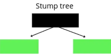
Now let us understand the workings of the Adaboost algorithm. As we know, the Adaboost algorithm uses decision stumps as a weak learner and these decision stumps are similar to the random forests which are not fully grown. There are three most important concepts about the working of the Ada boost algorithm.

1. Adaboost combines many stumps (weak learners) to build a strong predictive model.
2. Some stumps have more contribution to the final predictive model than others.
3. As the stumps are built in a sequence order so each stump tries to overcome the mistakes of the previous stump.

Considering the above points, here are the steps of the working of the Adaboost algorithm.

• The Adaboost algorithms assign the same weight value to the output as at the beginning every output value is equally important.
• After assigning the same weight, the Adaboost algorithm will create stump trees for each of the input attributes
• As stumps are simple decision trees, so based on the entropy value, the algorithm will select the stump tree that will have the lowest entropy value.
• And will compare the predictions of the selected stump trees with the actual value.
• The Adaboost algorithm will then increase the weights of all the misclassified values and will lower all weights of the correctly classified values.
• So, in the next iteration, the stump tree will give more attention to the prediction that has a higher weight value ( as they are misclassified values) and try to reduce the weight value (by classifying them correctly).
• The same iteration will continue unless we get really fewer values for weight or when the algorithm completes the maximum number of iterations.

Steps in Adaboost Implementation Using Python

We will be using the following simple steps to implement the Ada boost algorithm in Python.

• Exploring the data set and understanding it by using different visualization techniques.
• Splitting the dataset into the testing and training parts.
• Training the Ada boost model.
• Testing, evaluating, and visualizing the predictions of the model.

Later, we will also use various techniques for the hyperparameter tuning of the Ada boost algorithm.

Adaboost Classifier Using Python

Now we will use Python and its various well-known modules to implement the Ada boost algorithm on the classification dataset. We will be using the iris dataset from the sklearn module as a sample dataset and will train the Adaboost classifier.

Before going to the implementation part, make sure that you have installed the following Python modules as we will be using them in the implementation part.

• sklearn
• NumPy
• Pandas
• matplotlib
• seaborn
• plotly

You can use the pip command to install the required modules on your system.

Importing the Dataset

We will first import the submodule of the sklearn module to load the dataset. And then convert the dataset to a pandas DataFrame.

# importing the required modules
from sklearn import datasets
import pandas as pd
import numpy as np

# loading the iris dataset
dataset = datasets.load_iris()

# converting the data to DataFrame
data = pd.DataFrame(data= np.c_[dataset['data'], dataset['target']],
                     columns= dataset['feature_names'] + ['target'])

# printing the few rows
data.head()

This will show the input columns of the dataset. Now, let us visualize the dataset in various ways to know the hidden information.

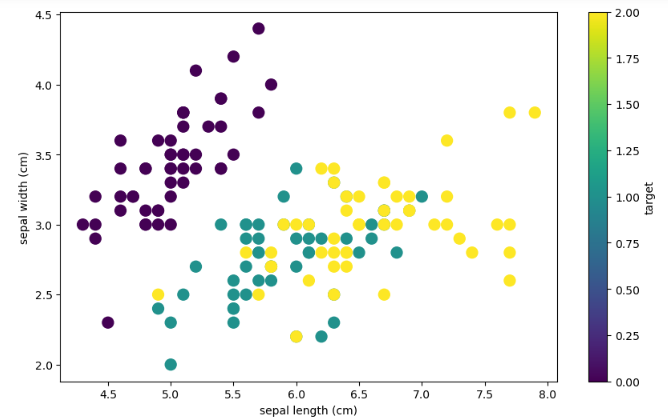
Let us first plot the scattered plot to see the distribution of the data points. This will help you to see the structure of the dataset based on the output values

# plotting the scatter plot based on coloring
data.plot.scatter(x="sepal length (cm)", y="sepal width (cm)", c='target', s=100, figsize=(10, 6))

Output:

Let us now plot the box plot to see if there are any outliers and it also helps us to see the shape of the distribution.

# plotting the box plot
data.drop('target', axis=1).plot.box(figsize=(10, 6))

Output:

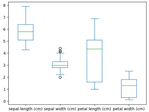
As you can see, except for the sepal width, there are no outliers in other attributes.

Splitting the Dataset

Now let us split the dataset into the testing and training parts. But before it, we have to divide the dataset into then input and output parts.

# splitting the dataset into input and output
Input = data.drop('target', axis=1)
Output =data['target']

The next part is to split the dataset into testing and training parts. The purpose of splitting the data into testing and training parts is that after training the model, we will use the testing data to evaluate the performance of the model. We will also assign value 1 to the random state.

# importing the module
from sklearn.model_selection import train_test_split

# splitting into testing and training parts
X_train, X_test, y_train, y_test = train_test_split(Input, Output, test_size=0.25, random_state=1)

We have assigned 25% of the total dataset to the testing part.

Training the Adaboost Classifier with 1 Stump Tree

First, we will use only 1 stump tree to train the Adaboost classifier and later will increase the number of stump trees.

Let us now import the model and initialize it.

# importing the classifier
from sklearn.ensemble import AdaBoostClassifier

# initailizing the ada boost classifier with 1 stump trees
Ada_clf = AdaBoostClassifier(n_estimators=1)

Let us now train the model on the training dataset.

# training the classifier
AdaBoost_2stump = Ada_clf.fit(X_train, y_train)

Once the training is complete, we can then move to the testing and validating part.

Testing and Evaluating the Classifier

Let us now make predictions using the testing dataset.

# making predictions
AdaBoost_pred = AdaBoost_2stump.predict(X_test)

Once, we have predictions then we can use various evaluation matrices to find out the performance of the model. Let us first use the confusion matrix to see the misclassified and correctly classified items.

# importing modules
import matplotlib.pyplot as plt
from sklearn.metrics import confusion_matrix, ConfusionMatrixDisplay

# confusion matrix plotting
cm = confusion_matrix(y_test,AdaBoost_pred, labels=Ada_clf.classes_)

# labelling
disp = ConfusionMatrixDisplay(confusion_matrix=cm, display_labels=Ada_clf.classes_)
disp.plot()
plt.show()

Output:

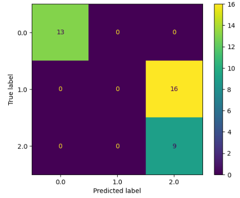
As you can see, there is a lot of misclassification in one of the categories. It is because of using only one stump tree. Let us also calculate the accuracy score.

# importing the module
from sklearn.metrics import accuracy_score

# printing
print("The accuracy is:  ", accuracy_score(y_test, AdaBoost_pred))

Output:

The accuracy is:   0.5789473684210527

As you can see, the accuracy is not too good.

Training Adaboost Classifier with 10 Stump Trees

Now we will increase the number of stump trees to 10 and see how the model will perform.

# initailizing the ada boost classifier with 10 stump trees
Ada_clf = AdaBoostClassifier(n_estimators=10)

# training the classifier
AdaBoost_10stump = Ada_clf.fit(X_train, y_train)

Once the training is complete, we can make predictions as we did before.

# making predictions
AdaBoost_pred = AdaBoost_10stump.predict(X_test)

Let us now again plot the confusion matrix.

# confusion matrix plotting
cm = confusion_matrix(y_test,AdaBoost_pred, labels=Ada_clf.classes_)

# labelling
disp = ConfusionMatrixDisplay(confusion_matrix=cm, display_labels=Ada_clf.classes_)
disp.plot()
plt.show()

Output:

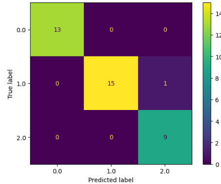
As you can see, this time the model was able to classify most of the items correctly. Let us also now find the accuracy score.

# printing
print("The accuracy is:  ", accuracy_score(y_test, AdaBoost_pred))

Output:

The accuracy is:   0.9736842105263158

As you can see, this time we get a much better accuracy score for the model.

Adaboost Regressor Using Python

It is not time to use the Ada boost algorithm on a regression dataset. The dataset that we are going to use is about the house prices in Dushanbe city.

Let us first import the dataset and get familiar with it.

# importing dataset 
data = pd.read_csv('house.csv')

# heading of the dataset
data.head()

Output:

number_of_rooms	floor	area	latitude	longitude	price
0	1	1	58.0	38.585834	68.793715	330000
1	1	14	68.0	38.522254	68.749918	340000
2	3	8	50.0	NaN	NaN	700000
3	3	14	84.0	38.520835	68.747908	700000
4	3	3	83.0	38.564374	68.739419	415000

As you can see, there are a few null values as well so let us remove null values.

# removing the null values
data.dropna(axis=0, inplace = True)

Now, our dataset is ready to be used to train the Ada boost algorithm.

Splitting the Dataset

Let us now divide the data set into input and output variables.

# input and output variables
Input = data.drop('price', axis=1)
Output = data.price

The next step is to split the dataset into the testing and training parts. We will also assign value 1 to the random state.

# importing the module
from sklearn.model_selection import train_test_split

# splitting into testing and training parts
X_train, X_test, y_train, y_test = train_test_split(Input, Output, test_size=0.25, random_state=1)

Once the splitting is complete, we can move to the training part of the model.

Training Adaboost Regressor Using Python

Let us first import the Adaboost regressor and initialize it with 20 stump trees.

# importing adaboost regressor
from sklearn.ensemble import AdaBoostRegressor

# Create adaboot with 20 stump trees
Ada_regressor = AdaBoostRegressor(n_estimators=20)

The next step is to train the model on the training dataset.

# training the adaboost regressor
AdaBoost_R = Ada_regressor.fit(X_train, y_train)

Once the training is complete, we can then move to the evaluation part.

Testing and Evaluating the Predictions of Regressor

Let us use the testing data to make predictions.

#Predict price 
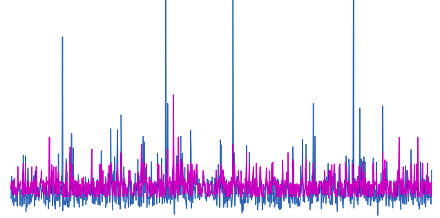
AdaBoost_pred = AdaBoost_R.predict(X_test)

Let us first visualize both the predictions and the actual values to see how well the predictions are.

#  fitting the size of the plot
plt.figure(figsize=(12, 8))

# plotting the graph for the actual values
plt.plot([i for i in range(len(y_test))],y_test, label="actual values")

# plotting the graph for predictions
plt.plot([i for i in range(len(y_test))],AdaBoost_pred, label="Predicted values", c='m')

plt.legend()
plt.show()

Output:

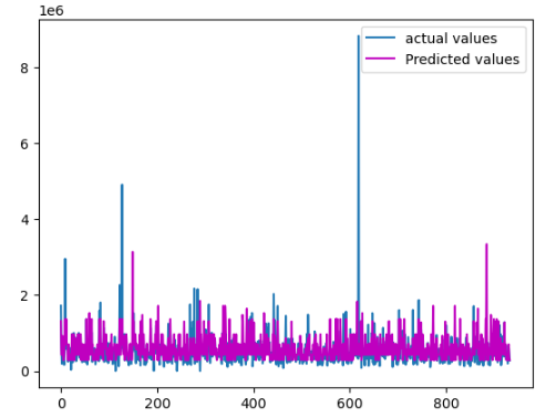
As you can see, the predictions are pretty much close to the actual values.

Hyperparameter Tuning of the Adaboost Algorithm

As we know the Adaboost has several important parameters that have a great role in the predictions and training of the model. In this section, we will explore some of these highly important parameters. We will again use the iris dataset. Let us import the dataset and then divide the data into inputs and outputs.

# loading the iris dataset
dataset = datasets.load_iris()

# converting the data to DataFrame
data = pd.DataFrame(data= np.c_[dataset['data'], dataset['target']],
                     columns= dataset['feature_names'] + ['target'])

# splitting the dataset into input and output
Input = data.drop('target', axis=1)
Output =data['target']

Now let us move to the important parameters and find out the optimum values.

The Optimum Number of Trees in Adaboost

As we know that Adaboost uses a decision stump as a weak learner so we have to find out the optimum number of decision stumps needed for the dataset. Let us first import all the necessary modules that we will be using in the hyperparameter tuning.

# importing all the necessary modules
from numpy import mean
from numpy import std
from sklearn.datasets import make_classification
from sklearn.model_selection import cross_val_score
from sklearn.model_selection import RepeatedStratifiedKFold
from matplotlib import pyplot

The next step is to create a function that will build various Ada boost models. And for the model, we will specify a different number of decision stumps starting from 50 to 1000.

# fuction to create models
def build_models():
    
#     dic of models
    Ada_models = dict()
    
	# number of decision stumps
    decision_stump= [10, 50, 100, 500, 1000]
        
#    using for loop to iterate though trees
    for i in decision_stump:
        
#         building model with specified trees
        models[str(i)] = AdaBoostClassifier(n_estimators=i)
    return models

The next step is to build a function for the validation of the models. In this case, we will use the cross-validation method. Let us build the function which returns the accuracy score of the models.

# function for the validation of model
def evaluate_model(model, Input, Ouput):
    
	# defining the method of validation
	cv = RepeatedStratifiedKFold(n_splits=10, n_repeats=3)
    
    
	# validating the model based on the accurasy score
	accuracy = cross_val_score(model, Input, Ouput, scoring='accuracy', cv=cv, n_jobs=-1)
    
#      accuracy score- hyperparameter tuning of Adaboost
	return accuracy

Now, we will call the above functions which will create the models and will evaluate them based on the accuracy score.

# calling the build_models function
models = build_models()

# creating list
results, names = list(), list()

# using for loop to iterate thoug the models
for name, model in models.items():
    
	# calling the validation function
	scores = evaluate_model(model, Input, Output)
    
    
	# appending the accuray socres in results
	results.append(scores)
	names.append(name)
    
    
	# printing results of hyperparameter tuning of Adaboost
	print('---->Stump tree (%s)---Accuracy( %.5f)' % (name, mean(scores)))

Output:

As you can see, the accuracy increases till 100 stump trees and then start decreasing maybe because the model starts overfitting after 100 stump trees. We can also visualize the above results using a box plot for each of the stump trees.

# plotting box plot of the 
pyplot.boxplot(results, labels=names,showmeans=True)

# showing the plot
pyplot.show()

Output:

As you can see that the mean accuracy is high when for 100 stump trees and then starts decreasing.

Tunning the Weak Learner in Ada Boost

A decision tree with one level is used as a weak learner by default in the Ada boost. We can increase the depth of the stump tree to get the optimum depth tree.

So, as we did before, we will create a function that will build models for various depth trees.

# building function for the model
def build_models():
    
#     creating dic of models
	models = dict()
    
#     specifying the depth of trees
	for i in range(1,8):
        
		# model
		base_model = DecisionTreeClassifier(max_depth=i)
        
		# creating dic of modles
		models[str(i)] = AdaBoostClassifier(base_estimator=base_model)
        
#   returining the model -results of hyperparameter tuning of Adaboost
	return models

In this section, we will not again build the evaluation function, as we have already created in the above section. So, we can use it here as well.

Let us now call the functions and find out the optimum depth for the weak learner of Ada Boost.

# calling the function
models = build_models()


# creating lists 
results, names = list(), list()

# iterating through the models
for name, model in models.items():
    
	# calling the evalution function
    accuracy = evaluate_model(model, Input, Output)
    
	# appending the results
    results.append(accuracy)
    names.append(name)
	
#     printing results of hyperparameter tuning of Adaboost
    print('---->Stump tree (%s)---Accuracy( %.5f)' % (name, mean(accuracy)))

Output:

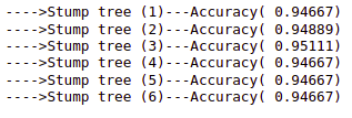
As you can see, the accuracy increases to 3 depth and then starts decreasing. So, the optimum depth for weak learners is 3.

Let us also plot the box plot of our findings.

# plotting box plot of the 
pyplot.boxplot(results, labels=names,showmeans=True)

# showing the plot
pyplot.show()

Output:

As you can see, when the decision tree depth was 3, we have the highest accuracy score.

Tuning the Learning rate in Ada Boost

The learning rate is simply the step size of each iteration. The default value of the learning rate in the Ada boost is 1. We will now use the hyperparameter tuning method to find the optimum learning rate for our model.

Similar to another step of tuning, first we will create a function that will create multiple models with different values of learning rate.

# building the models
def build_models():
    
#     creating the model dic
	models = dict()
    
    
	# learning rate for various values
	for i in arange(0.1, 2.1, 0.1):
		key = '%.3f' % i
        
#         models in dic
		models[key] = AdaBoostClassifier(learning_rate=i)
    
#     returning models -results of hyperparameter tuning of Adaboost
	return models

We will use the same previous model evaluating function and call it.

# calling the function
models = build_models()

# creating the list
results, names = list(), list()

# for loop to iterate through the models
for name, model in models.items():
    
    
	# calling the evaluting function
	accuracy = evaluate_model(model, Input, Output)
	
#     storing the accurcy
	results.append(accuracy)
	names.append(name)
	
#     printing results of hyperparameter tuning of Adaboost
	print('---->Stump tree (%s)---Accuracy( %.5f)' % (name, mean(accuracy)))

Output:

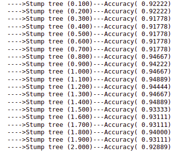
As you can see that we have optimum accuracy when the learning rate was equal to 1.1 and 1.4.

Let us now also visualize the mean of accuracy using a box plot.

# fixing the size
pyplot.figure(figsize=(10, 8))

# plotting the values
pyplot.boxplot(results, labels=names, showmeans=True)
pyplot.show()

Output:

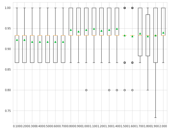
As you can see, the mean accuracy is high for values 1.1 and 1.4.

Hyperparameter Tuning of Adaboost Using GridSearchCV

Now, we will use the GridSearchCV method to find the optimum values for the parameters of the Ada boost algorithm using the same dataset. GridSearchCV takes every possible value ( specified ones) and train the model on the different combination and returns the optimum values.

# defining the classifier
model = AdaBoostClassifier()

# creating a dic for the grid
grid = dict()

# estimator till 500
grid['n_estimators'] = [10, 50, 100, 200, 500]

# defining learning rate
grid['learning_rate'] = [0.0001, 0.01, 0.1, 1.0, 1.1, 1.2]


# defining the CV
cv = RepeatedStratifiedKFold(n_splits=10, n_repeats=3)

# initializing the grid search
grid_search = GridSearchCV(estimator=model, param_grid=grid, n_jobs=-1, cv=cv, scoring='accuracy')


# training the model on grid search for hyperparameter tuning of Adaboost
grid_result = grid_search.fit(Input, Output)

# finding the best results /hyperparameter tuning of Adaboost
print("Best: %f using %s" % (grid_result.best_score_, grid_result.best_params_))

Output:

As you can see the combination of 100 estimators and a 1.0 learning rate provides optimum results according to GridSearchCV.

NOTE: You can get access to all the source code and the dataset from my GitHub account. Please don’t forget to give it a star and follow.

Summary

Ada boost algorithm is a type of supervised machine learning boosting algorithm that can be used for both classification and regression problems. The Ada boost can use any classifier as a weak learner and combine them to form an optimum model but the most commonly used weak classifier in the Ada boost algorithm is the one-level decision tree known as the decision stump. In this article, we discussed how the Ada boost algorithm works and is implemented using Python on classification and regression datasets. Moreover, we also learned Hyperparameter Tuning of the Adaboost using various methods.

Frequently Asked Questions

Is Ada Boost a supervised machine learning algorithm?

Yes, the Ada boost algorithm, very much similar to any other boosting algorithm is a supervised machine learning algorithm and the model can be trained using the training dataset containing the output values.

How does the Ada boost algorithm work?

The Ada boost algorithm works by training many weak learners. In this case, the weak learners are the stump trees. So, each stump tree tries to reduce the prediction errors of the previous trees.

Is ada boost better than XGBoost?

XGboost is much faster and smarter than the Ada Boost algorithm.

How to apply ada boost to my dataset

First, divide the dataset into the testing and training parts. Then import the Adaboost ( classifier or regression) and train the model on the training dataset. Once the training is complete, you can then use the testing part of the dataset to test the model.

Is XGBoost the same as ada boost?

The answer is no. Yes, they both are boosting algorithms but they are not similar.

Where we can use Ada boost?

The Ada boost algorithm can be used for both classification and regression datasets.

Is ada boost a good option for boosting?

Yes, Ada boost is considered to be the very first boosting algorithm. But mostly the selection of an algorithm depends on your dataset.