Did you wonder how can you apply the ARIMA model in Python for non-stationary time series? Although the ARIMA model in Python is very efficient for the stationary time series, we can also use the ARIMA model for nonstationary time series as well.
A statistical model called ARIMA is applied to time series analysis. The ARMA model, which is used for stationary time series, is generalized by the ARIMA model. Non-stationary time series can employ the ARIMA model, but you must first differentiate them. In this article, we will learn how we can apply the ARIMA model in Python to non-stationary time series. We already assume that you have basic knowledge of machine learning and its various algorithms. In this short article, we will discuss how we can use the ARIMA model in Python for non-stationary time series. We will use various Python modules to visualize the results.
What is the ARIMA Model in Python?
ARIMA models provide another approach to time series forecasting which aim to describe the autocorrelations in the data. It stands for AutoRegressive Integrated Moving Average. Based on previous time series values, it is used to predict future time series values. Both stationary and non-stationary time series can be modeled using the ARIMA model but our focus in this article will be to apply the ARIMA model to non-stationary time series. Check Sklearn One Hot Encoder Examples (Single and Multiple Columns)
Typically, ARIMA models are written as ARIMA (p, d, q), where p denotes the order of the autoregressive model (AR), d is the level of differencing, and q denotes the order of the moving-average model (MA). A non-stationary time series is transformed into a stationary one using differencing in the ARIMA model, which then uses historical data to forecast future values. In order to predict future values, the model applies “auto” correlations and moving averages to residual errors in the data.
How to Convert Non-stationary Time Series to Stationary Time Series.
A stationary time series is one whose characteristics are independent of the observation time. Time series with trends or seasonality are therefore not stationary because the trend and seasonality will change the time series’ value at different points in time. A white noise series, on the other hand, is stationary; regardless of the time you examine it, it should appear about the same.
A non-stationary time series can be made stationary in a variety of methods. Using the log, square, square root, cube, cube root, and many other practical approaches are a few examples. In this article, we will take the following methods to convert the non-stationary time series to a stationary time series.
- Log scale transformation
- Timeshift transformation
Now, let us use Python to implement the mentioned methods and convert a non-stationary time series to a stationary time series.
Non-stationary Time Series to Stationary Times Series
In this article, we will be using a dataset about Bitcoin and will use various methods to convert the Bitcoin dataset into a stationary dataset. Let us first import the dataset and then use print a few rows to get familiar with the dataset.
# importing the module
import pandas as pd

# importing the dataset
data = pd.read_csv("BTC-USD.csv")
The dataset contains information about many factors. We only need the Date and Closing price of the Bitcoin. So, we will remove all other columns.
# removing few columns
data.drop("Open", inplace = True, axis = 1)
data.drop("High", inplace = True, axis = 1)
data.drop("Low", inplace = True, axis = 1)
data.drop("Adj Close", inplace = True, axis = 1)
data.drop("Volume", inplace = True, axis = 1)
Now we are good to go to analyze the dataset.
How to Check if the Time Series is Stationary?
There can be many ways to check if the time series is stationary or not. The simplest way is to find the mean and standard deviations and if they are constant, that means the time series is stationary.
Let us then find the mean and standard deviation of the Bitcoin dataset.
# finding the rolling mean and std
mean = data.rolling(window=12).mean()
std = data.rolling(window=12).std()
A rolling mean is simply the mean of a certain number of previous periods in a time series. The above piece of code has calculated the rolling mean and standard deviation. The window size represents the size of the rolling mean on each interval.
Let us now plot the rolling mean and standard deviation on a plot so that it will be easy to see if they are constant.
# importing the required modules
import matplotlib.pyplot as plt

#Plot rolling statistics
mean = plt.plot(mean, color='red', label='Rolling Mean')
std = plt.plot(std, color='green', label='Rolling Std')

# labeling the axis
plt.legend(loc='best')
plt.title('Rolling Mean and Std')
plt.show()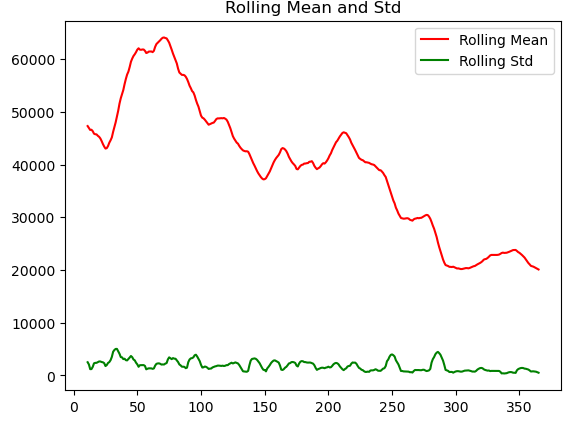
The standard deviation is nearly constant but the mean is not constant which means the time series is nonstationary, so we will use different methods to make it stationary.
Log Scale Transformation Using Python
Among the various forms of transformations used to change skewed data to roughly adhere to normality, the log transformation is likely the most common. The log-transformed data has a normal or very close to normal distribution if the original data has a log-normal distribution or something similar. Or in simple words, Log transformation is a data transformation method in which it replaces each variable x with a log(x).
Let us now apply the log scale transformation to our dataset to make it a stationary time series using Python.
# importing the module
import numpy as np

#Applying the log transformation on Closing price
logScale = np.log(data['Close'])

#TFinding the average and std
moving_Average = logScale.rolling(window=12).mean()
moving_STD = logScale.rolling(window=12).std()

# plotting the graph
plt.plot(logScale)
plt.plot(moving_Average, color='red')
plt.show()
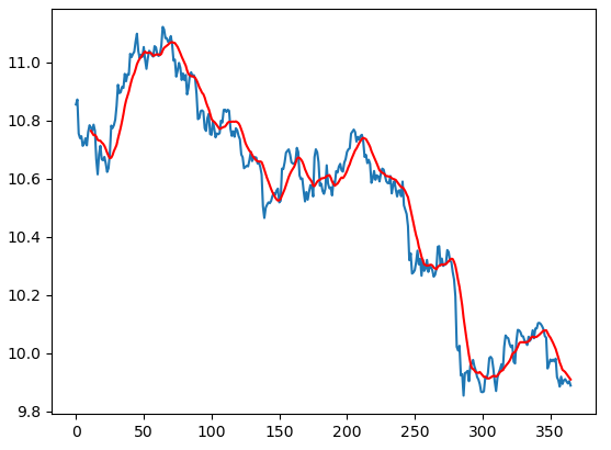
We currently have the time series’ log(x) values. Therefore, we can construct a function that subtracts the rolling mean and the mean of the log scale, resulting in a constant mean, to make the dataset stationary.
Let us now transform the time series dataset into the new one.
# transforming the time series
log_transformed = logScale - moving_Average

#Remove NAN values
log_transformed.dropna(inplace=True)

# printing heading of dataset
log_transformed.head()
As we now have the transformed time series. Let us now find the rolling mean and std and then will again visualize the time series to see if the data is now stationary.
# fixing the size of image
plt.figure(figsize=[10, 6])

# finding the rolling mean and std
movingAverage = log_transformed.rolling(window=12).mean()
movingSTD = log_transformed.rolling(window=12).std()

# plotting graph and meaa and std
orig = plt.plot(log_transformed, color='blue', label='Original')
mean = plt.plot(movingAverage, color='red', label='Rolling Mean')
std = plt.plot(movingSTD, color='black', label='Rolling Std')

# plotting stationary time series data
plt.legend(loc='best')
plt.title('Rolling Mean & Std')
plt.show()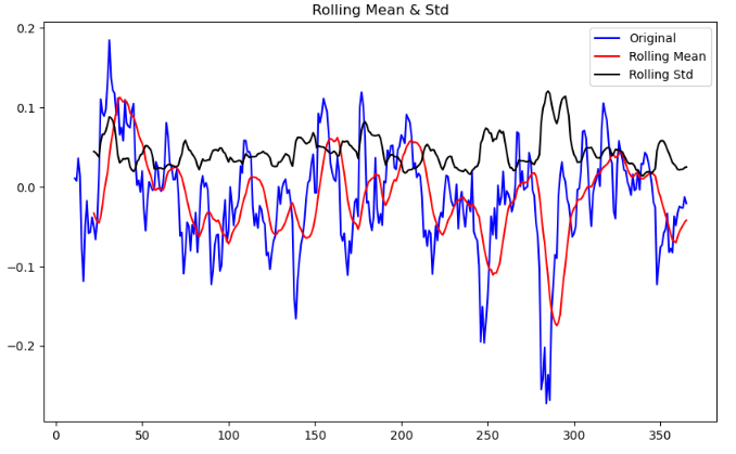
This time, instead of going up, the mean is going in a constant direction which is horizontal and the time series is more stationary than the previous one.
Timeshift Transformation Using Python
Timeshift transformation is another method through which we can convert a stationary time series to a nonstationary one. Let us first apply the timeshift transformation on the time series dataset and then visualize it.
# fixing the size of image
plt.figure(figsize=[10, 6])

#  applynig timeshift transformation
Shifting = logScale - logScale.shift()

# plotting the timeshif
plt.plot(Shifting , c='m')

# showing the timeshift
plt.show()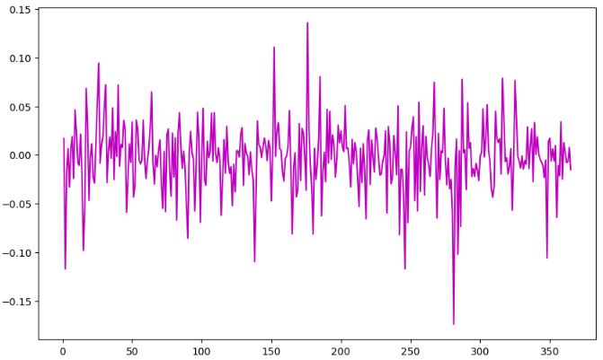
The data has been transformed horizontally. To check, if the data is not stationary, we will again find the rolling mean and standard deviation and will plot them on a graph.
# fixing the size of image
plt.figure(figsize=[10, 6])

#rolling mean of timeshift transformed data
moving_Average = Shifting.rolling(window=12).mean()

# rolling std of timeshift transformed data
moving_STD = Shifting.rolling(window=12).std()

#plotting the original data
orig = plt.plot(Shifting, color='blue', label='Original')

# plotting the mean and std of transformed data
mean = plt.plot(moving_Average, color='red', label='Rolling Mean')
std = plt.plot(moving_STD, color='black', label='Rolling Std')

# Labeling
plt.legend(loc='best')
plt.title('Rolling Mean & Std')
plt.show()
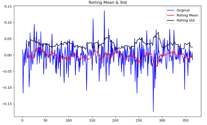
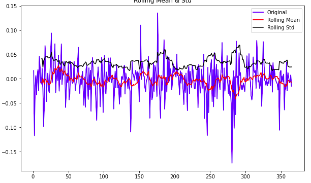
This time the standard deviation and mean are nearly constant suggesting that the time series is now stationary.
You can access the source code from my GitHub account. Please don’t forget to give me a star and follow.
Learn how to train the Arima model in Python by going through the article which explains the concepts of the Arima model.
Summary
An autoregressive integrated moving average, or ARIMA, is a statistical analysis model that uses time series data to either better understand the data set or to predict future trends. In this article, we discuss how we can use various methods on times series to convert the nonstationary time series to stationary one so that we can apply the ARIMA model in Python easily as the ARIMA model in Python only works on stationary time series

